stat220-spring24 – Cross Validation and Linear Regression

Resampling methods

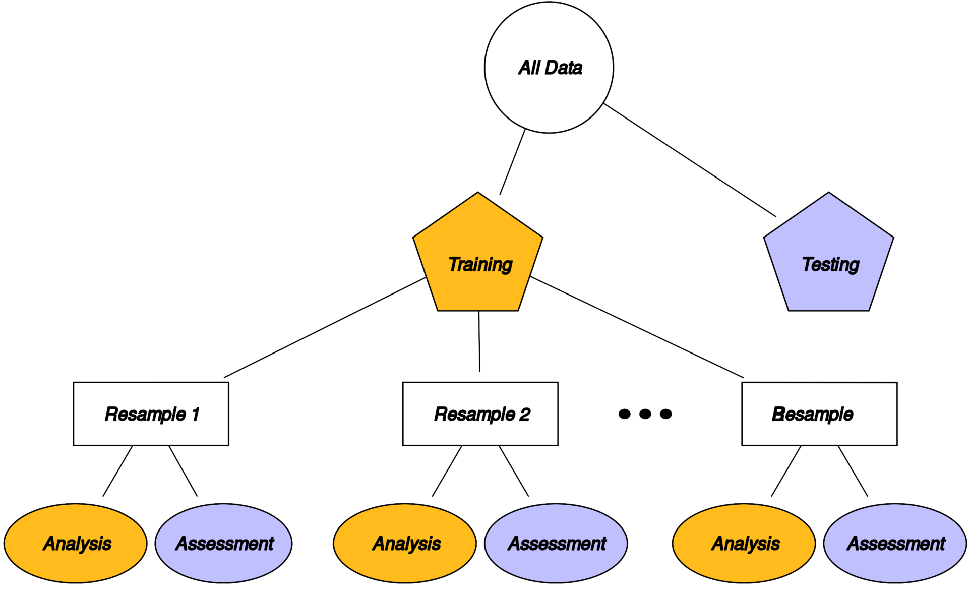
Create a series of data sets similar to the training/testing split, always used with the training set

Kuhn and Johnson (2019)

Why not to use single (training) test set

Cross validation

Idea: Split the training data up into multiple training-validation pairs, evaluate the classifier on each split and average the performance metrics

Image courtesy of Dennis Sun

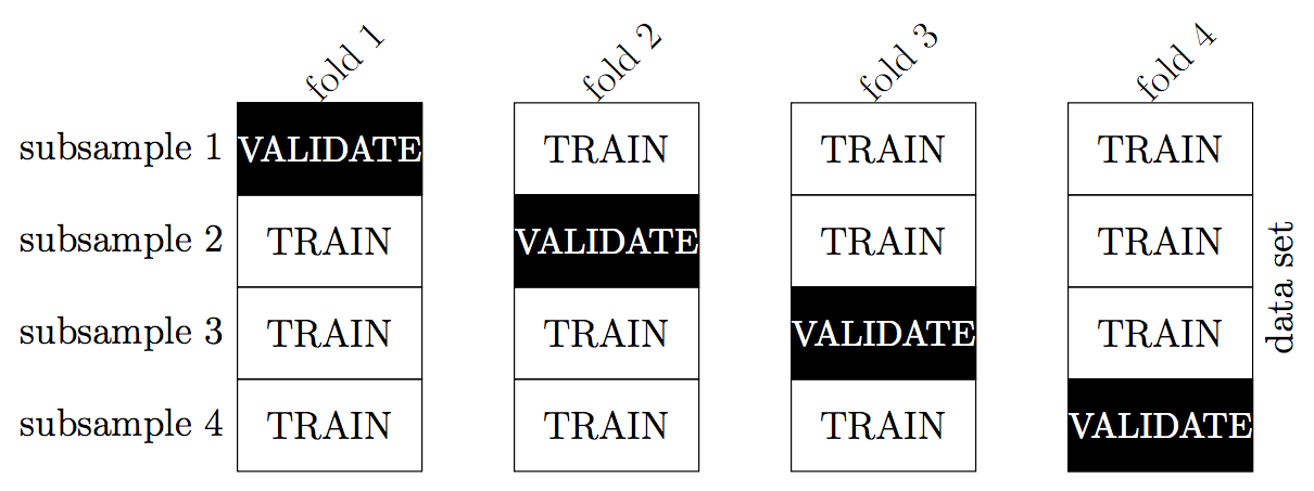
k-fold cross validation

split the data into $k$ subsets
combine the first $k-1$ subsets into a training set and train the classifier
evaluate the model predictions on the last (i.e. $k$ th) held-out subset
repeat steps 2-3 $k$ times (i.e. $k$ “folds”), each time holding out a different one of the $k$ subsets
calculate performance metrics from each validation set
average each metric over the $k$ folds to come up with a single estimate of that metric

5-fold cross validation

Creating the recipe

fire_recipe <- recipe(classes ~  temperature + isi, data = fire_train) %>%
  step_scale(all_predictors()) %>%
  step_center(all_predictors())

5-fold cross validation

Create your model specification and use tune() as a placeholder for the number of neighbors

knn_spec <- nearest_neighbor(mode = "classification",
                             engine = "kknn",
                             weight_func = "rectangular", 
                             neighbors = tune())

Split the fire_train data set into v = 5 folds, stratified by classes

# replicate 5-fold cross-validation 10 times
fire_vfold <- vfold_cv(fire_train, v = 5, strata = classes, repeats = 10)

5-fold cross validation

Create a grid of $K$ values, the number of neighbors

k_vals <- tibble(neighbors = seq(from = 1, to = 40, by = 1))

Run 5-fold CV on the k_vals grid, storing four performance metrics

knn_fit <- workflow() %>%
  add_recipe(fire_recipe) %>%
  add_model(knn_spec) %>%
  tune_grid(resamples = fire_vfold, 
            grid = k_vals,
            metrics = metric_set(accuracy, sensitivity, specificity, ppv))

Choosing K

Collect the performance metrics

cv_metrics <- collect_metrics(knn_fit)
cv_metrics %>% head(6)

# A tibble: 6 × 7
  neighbors .metric     .estimator  mean     n std_err .config              
      <dbl> <chr>       <chr>      <dbl> <int>   <dbl> <chr>                
1         1 accuracy    binary     0.987    50 0.00343 Preprocessor1_Model01
2         1 ppv         binary     0.999    50 0.00133 Preprocessor1_Model01
3         1 sensitivity binary     0.979    50 0.00586 Preprocessor1_Model01
4         1 specificity binary     0.998    50 0.002   Preprocessor1_Model01
5         2 accuracy    binary     0.987    50 0.00343 Preprocessor1_Model02
6         2 ppv         binary     0.999    50 0.00133 Preprocessor1_Model02

Choosing K

Collect the performance metrics and find the best model

cv_metrics %>%
  group_by(.metric) %>%
  slice_max(mean)

# A tibble: 20 × 7
# Groups:   .metric [4]
   neighbors .metric     .estimator  mean     n std_err .config              
       <dbl> <chr>       <chr>      <dbl> <int>   <dbl> <chr>                
 1         1 accuracy    binary     0.987    50 0.00343 Preprocessor1_Model01
 2         2 accuracy    binary     0.987    50 0.00343 Preprocessor1_Model02
 3        11 ppv         binary     1        50 0       Preprocessor1_Model11
 4        12 ppv         binary     1        50 0       Preprocessor1_Model12
 5        13 ppv         binary     1        50 0       Preprocessor1_Model13
 6        14 ppv         binary     1        50 0       Preprocessor1_Model14
 7        15 ppv         binary     1        50 0       Preprocessor1_Model15
 8        16 ppv         binary     1        50 0       Preprocessor1_Model16
 9        17 ppv         binary     1        50 0       Preprocessor1_Model17
10        18 ppv         binary     1        50 0       Preprocessor1_Model18
11         1 sensitivity binary     0.979    50 0.00586 Preprocessor1_Model01
12         2 sensitivity binary     0.979    50 0.00586 Preprocessor1_Model02
13        11 specificity binary     1        50 0       Preprocessor1_Model11
14        12 specificity binary     1        50 0       Preprocessor1_Model12
15        13 specificity binary     1        50 0       Preprocessor1_Model13
16        14 specificity binary     1        50 0       Preprocessor1_Model14
17        15 specificity binary     1        50 0       Preprocessor1_Model15
18        16 specificity binary     1        50 0       Preprocessor1_Model16
19        17 specificity binary     1        50 0       Preprocessor1_Model17
20        18 specificity binary     1        50 0       Preprocessor1_Model18

Choosing K: Visualization

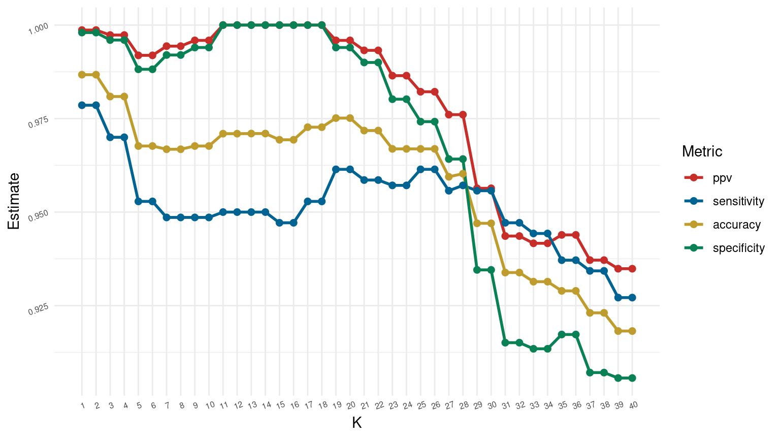
The full process

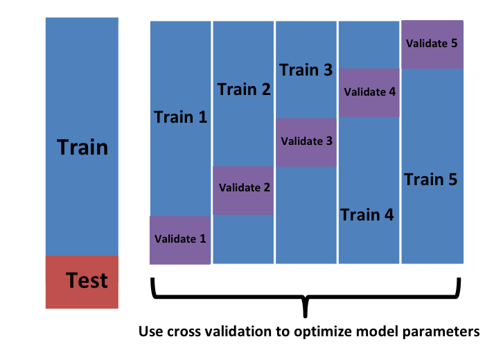
Image source: rafalab.github.io/dsbook/

Please clone the ca23-yourusername repository from Github
Please do problem 1 in the class activity for today

10:00

Supervised Learning

Supervised learning: Learning a function that maps an input to an output based on example inputoutput pairs.
Function: $\mathrm{y}=\mathrm{f}(\mathrm{x})$ , where $\mathrm{y}$ is the label (output) we predict, and $\mathrm{x}$ is the feature(s) (input).
Goal: Find a function that calculates $y$ from $x$ values accurately for all cases in the training dataset.

Linear Regression: The Basics

Linear regression fits a linear equation to observed data to describe the relationship between variables.

$y=\beta_0 + \beta_1x_1 + \beta_2x_2 + \cdots + \epsilon$

$y$ is the dependent variable (what we’re trying to predict),
$x_1, x_2, \cdots$ are independent variables (features),
$\beta_0, \beta_1, \beta_2, \cdots$ are coefficients, and $\epsilon$ represents the error term.

Objective: Minimize the differences between the observed values and the values predicted by the linear equation.

Relevant Metrics

$\text{MSE} =\frac{1}{n} \sum_{i=1}^n\left(y_i-\hat{y}_i\right)^2$

$\text{RMSE} =\sqrt{\frac{1}{n} \sum_{i=1}^n\left(y_i-\hat{y}_i\right)^2}$

$R^2 = 1 - \frac{\sum_{i=1}^{n} (y_i - \hat{y}_i)^2}{\sum_{i=1}^{n} (y_i - \overline{y})^2}$

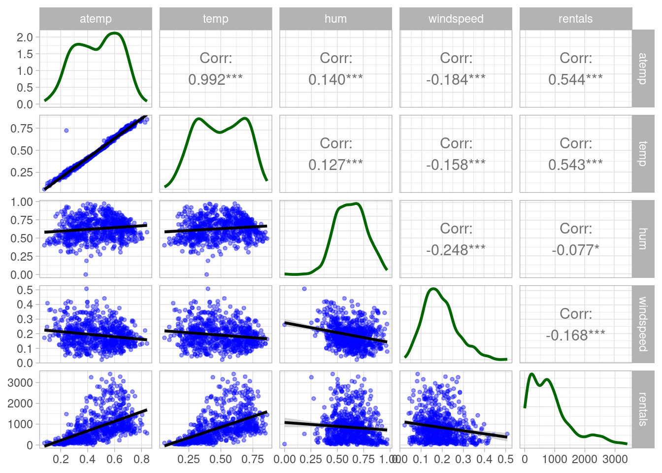
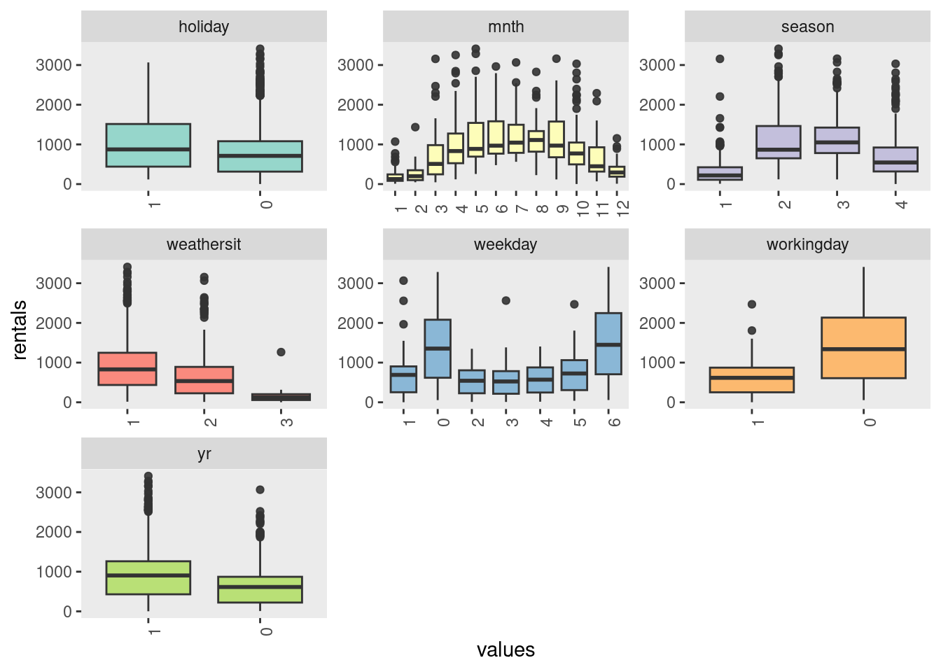
Case study: Bike Share Scheme

Data from a real study on a bicycle sharing scheme was collected to predict rental numbers based on seasonality and weather conditions.

season	mnth	weekday	workingday	weathersit	temp	atemp	hum	windspeed	rentals
1	1	6	0	2	0.344167	0.363625	0.805833	0.160446	331
1	1	0	0	2	0.363478	0.353739	0.696087	0.248539	131
1	1	1	1	1	0.196364	0.189405	0.437273	0.248309	120
1	1	2	1	1	0.200000	0.212122	0.590435	0.160296	108
1	1	3	1	1	0.226957	0.229270	0.436957	0.186900	82

Variable	Description
instant	An identifier for each unique row
season	Encoded numerical value for the season (1 for spring, 2 for summer, 3 for fall, 4 for winter)
yr	Observation year in the study, spanning two years (0 for 2011, 1 for 2012)
mnth	Month of observation, numbered from 1 (January) to 12 (December)
holiday	Indicates if the observation was on a public holiday (binary value)
weekday	Day of the week of the observation (0 for Sunday to 6 for Saturday)
workingday	Indicates if the day was a working day (binary value, excluding weekends and holidays)
weathersit	Weather condition category (1 for clear, 2 for mist/cloud, 3 for light rain/snow, 4 for heavy rain/hail/snow/fog)
temp	Normalized temperature in Celsius
atemp	Normalized “feels-like” temperature in Celsius
hum	Normalized humidity level
windspeed	Normalized wind speed
rentals	Count of bicycle rentals recorded

Descriptive Statistics
Code

variable	Min.	1st Qu.	Median	Mean	3rd Qu.	Max.
atemp	0.079070	0.337842	0.486733	0.474354	0.608602	0.840896
temp	0.059130	0.337083	0.498333	0.495385	0.655417	0.861667
hum	0.000000	0.520000	0.626667	0.627894	0.730209	0.972500
windspeed	0.022392	0.134950	0.180975	0.190486	0.233214	0.507463
rentals	2.000000	315.500000	713.000000	848.176471	1096.000000	3410.000000

bike %>%
  select(atemp,temp, hum, windspeed, rentals) %>%
  map_df(~summary(.), .id = "variable") %>%
  mutate(across(-variable, round, digits = 6))

Data preparation and train-test split

set.seed(2056)
bike_select <- bike %>% 
  select(c(season, mnth, holiday, weekday, workingday, weathersit,
           temp, atemp, hum, windspeed, rentals)) %>% 
    mutate(across(1:6, factor))


bike_split <- bike_select %>% 
  initial_split(prop = 0.75, strata = holiday) 

bike_train <- training(bike_split)
bike_test <- testing(bike_split)

Model specification

lm_spec <- # your model specification
  linear_reg() %>%  # model type
  set_engine(engine = "lm") %>%  # model engine
  set_mode("regression") # model mode

Fit the model

# Train a linear regression model
lm_mod <- lm_spec %>% 
  fit(rentals ~ ., data = bike_train)

glance(lm_mod$fit) %>% knitr::kable()

r.squared	adj.r.squared	sigma	statistic	p.value	df	logLik	AIC	BIC	deviance	df.residual	nobs
0.6956614	0.6798592	385.1778	44.02308	0	27	-4025.838	8109.677	8234.559	77148225	520	548

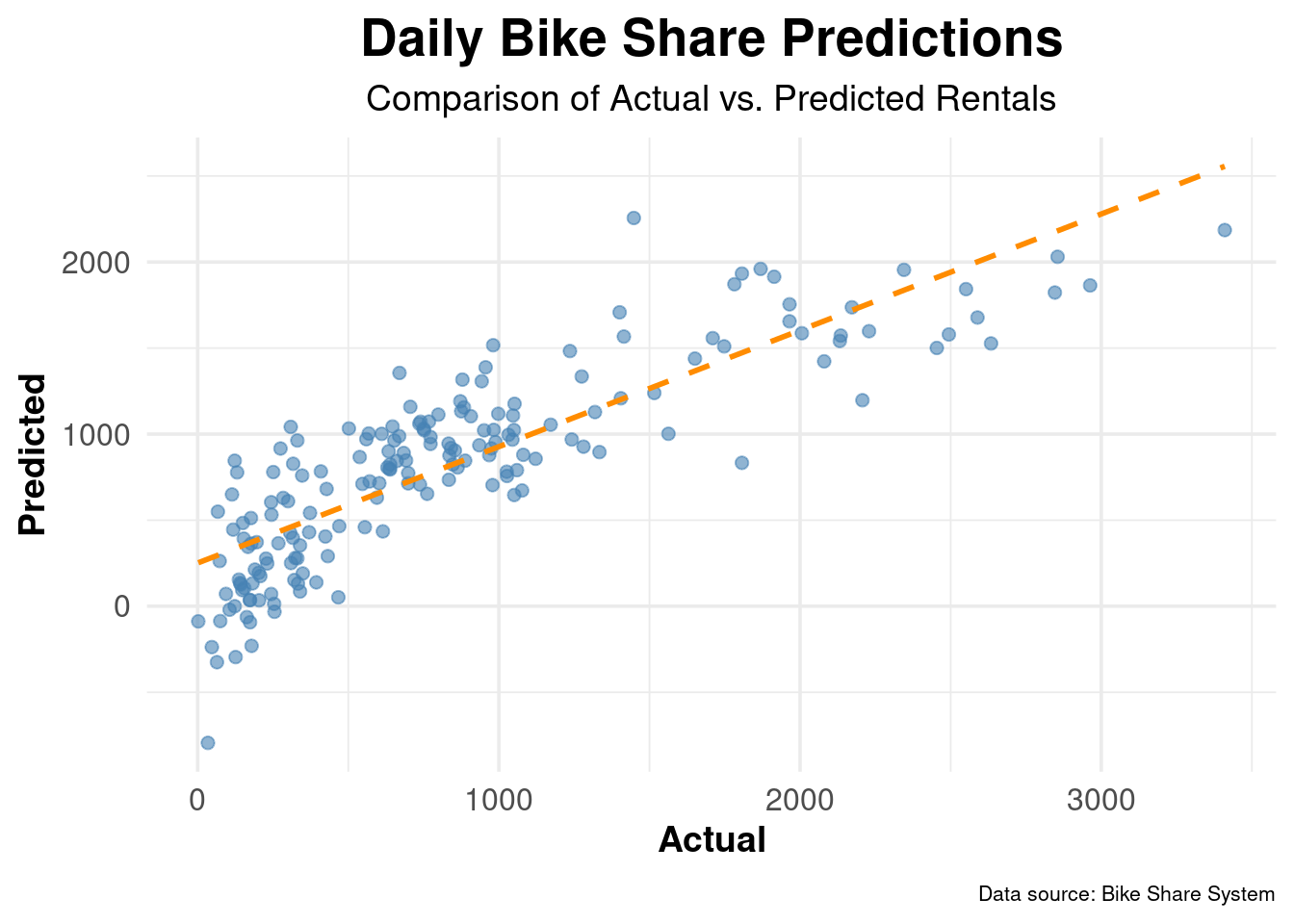
Predict on test data

results <- bike_test %>% 
  bind_cols(lm_mod %>% 
    predict(new_data = bike_test)) %>% 
      select(c(rentals, .pred))

results %>% slice_head(n =6)

# A tibble: 6 × 2
  rentals .pred
    <dbl> <dbl>
1     331 963. 
2     131 778. 
3     148  93.8
4     251 779. 
5      75 -86.4
6     150 484.

Evaluate the model

eval_metrics <- metric_set(rmse, rsq)

# Evaluate RMSE, R2 based on the results
eval_metrics(data = results,
             truth = rentals,
             estimate = .pred) %>% 
  select(-2)

# A tibble: 2 × 2
  .metric .estimate
  <chr>       <dbl>
1 rmse      380.   
2 rsq         0.710

Please finish the remaining problems in the class activity for today

10:00