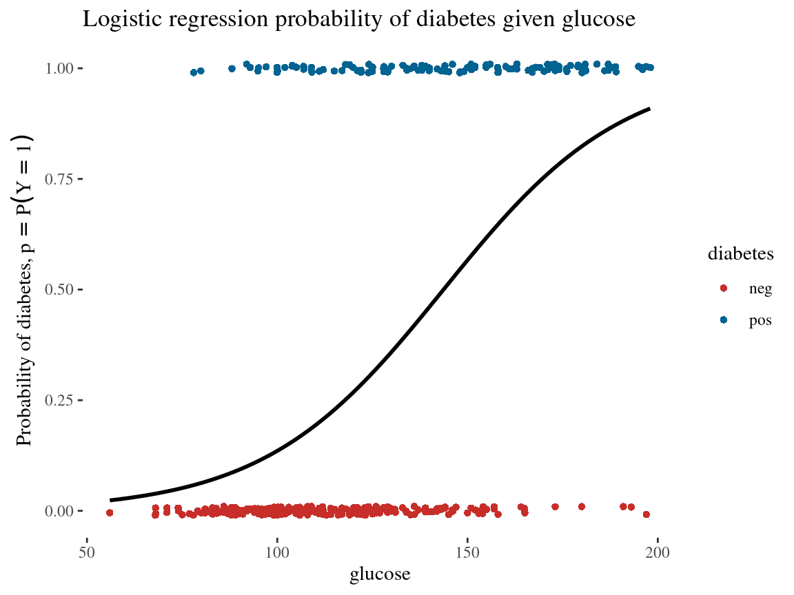
Logistic Regression
STAT 220
Group Activity 1

- Please clone the
ca24-yourusernamerepository from Github - Please do problem 1 in the class activity for today
10:00 Threshold for classification
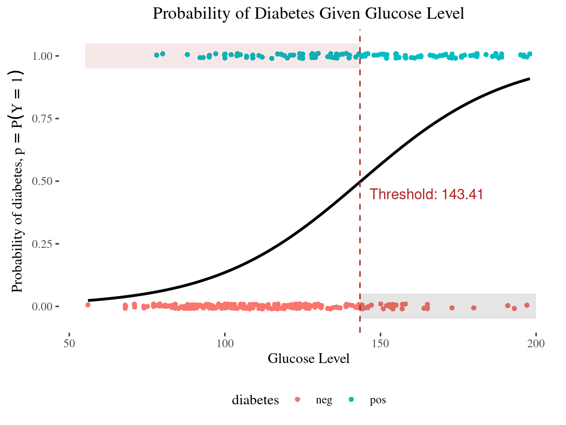
Class Prediction
Custom Metrics
custom_metrics <- metric_set(accuracy,
                             sensitivity,
                             specificity,
                             ppv)
custom_metrics(db_results,
               truth = diabetes,
               estimate = .pred_class)
# A tibble: 4 × 3
.metric .estimator .estimate
<chr> <chr> <dbl>
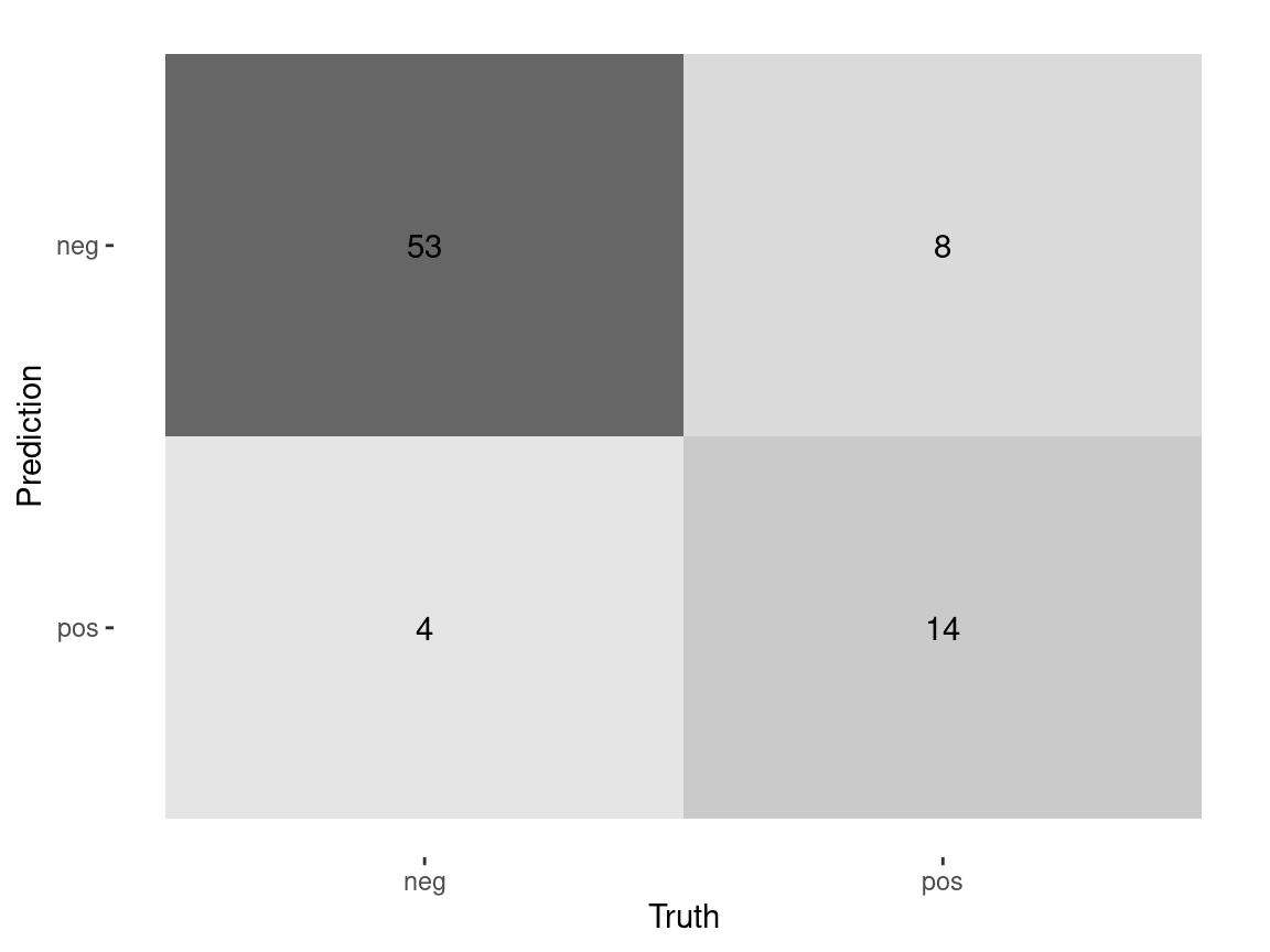
1 accuracy binary 0.823
2 sensitivity binary 0.982
3 specificity binary 0.409
4 ppv binary 0.812Custom Metrics

custom_metrics <- metric_set(accuracy,
                             sensitivity,
                             specificity,
                             ppv)
custom_metrics(db_results,
               truth = diabetes,
               estimate = .pred_class)
# A tibble: 4 × 3
.metric .estimator .estimate
<chr> <chr> <dbl>
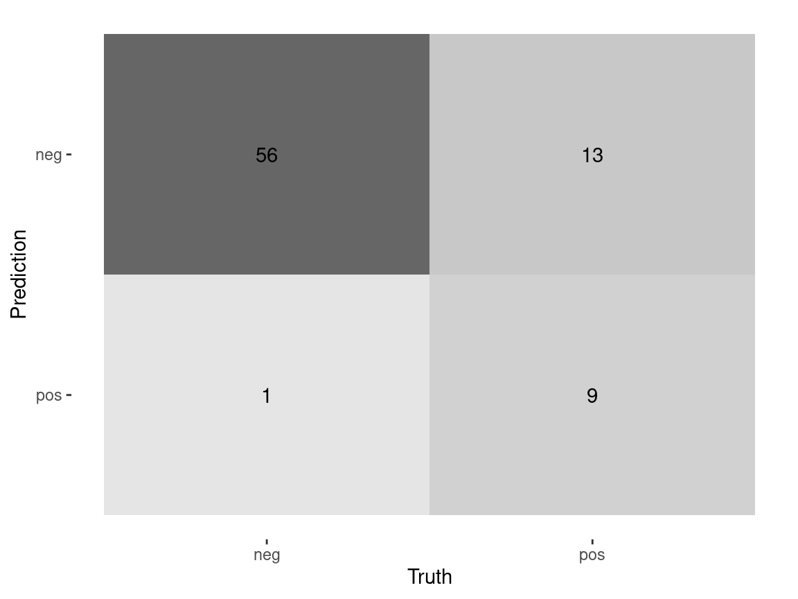
1 accuracy binary 0.785
2 sensitivity binary 0.754
3 specificity binary 0.864
4 ppv binary 0.935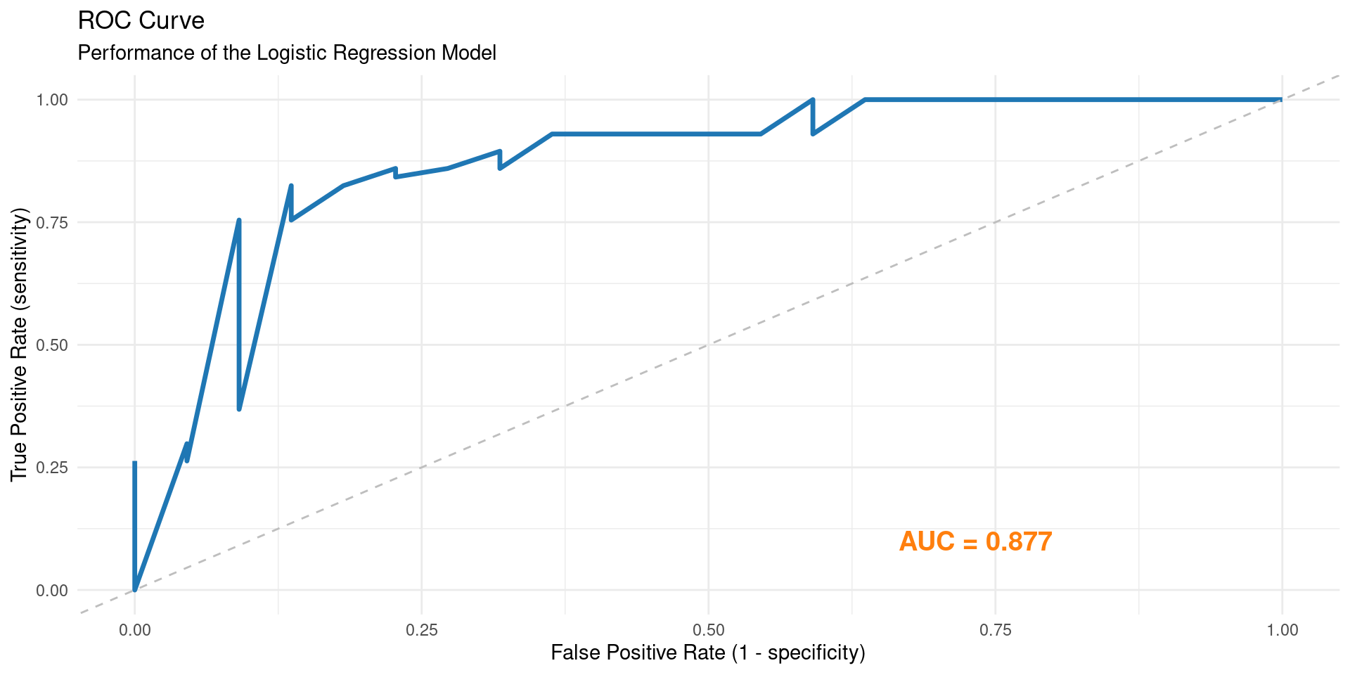
library(yardstick)

diabetes_prob <- predict(fitted_logistic_model, db_test, type = "prob")
diabetes_results <- db_test %>% select(diabetes) %>% bind_cols(diabetes_prob)

diabetes_results %>%
  roc_curve(truth = diabetes, .pred_neg) %>%
  ggplot(aes(x = 1 - specificity, y = sensitivity)) +
  geom_line(color = "#1f77b4", size = 1.2) +
  geom_abline(linetype = "dashed", color = "gray") +
  annotate("text", x = 0.8, y = 0.1, label = paste("AUC =", round(roc_auc(diabetes_results, truth = diabetes, .pred_neg)$.estimate, 3)), hjust = 1, color = "#ff7f0e", size = 5, fontface = "bold") +
  labs(title = "ROC Curve", subtitle = "Performance of the Logistic Regression Model", x = "False Positive Rate (1 - specificity)", y = "True Positive Rate (sensitivity)") +
theme_minimal()Group Activity 2
- Please finish the remaining problems in the class activity for today
10:00