Factor manipulations

STAT 220

Bastola

Factors - categorical data

See forcats cheatsheet and forcats vignette

Example - specify levels fct_relevel()

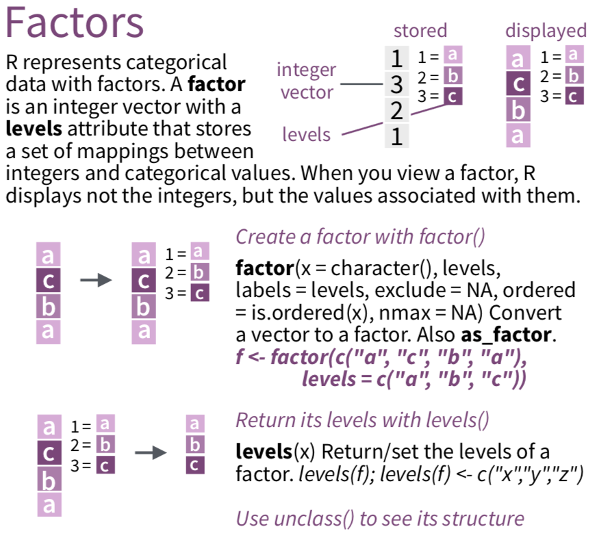
mydata <- tibble(
  id = 1:4, 
  grade=c("9th","10th","11th","9th")) %>%
  mutate(grade_fac = factor(grade)) 
levels(mydata$grade_fac)

[1] "10th" "11th" "9th" 

mydata %>% 
  arrange(grade_fac)

# A tibble: 4 × 3
     id grade grade_fac
  <int> <chr> <fct>    
1     2 10th  10th     
2     3 11th  11th     
3     1 9th   9th      
4     4 9th   9th      

mydata <- mydata %>% 
  mutate(
    grade_fac = 
      fct_relevel(grade_fac, 
                  c("9th","10th","11th"))) 
levels(mydata$grade_fac)

[1] "9th"  "10th" "11th"

mydata %>% arrange(grade_fac)

# A tibble: 4 × 3
     id grade grade_fac
  <int> <chr> <fct>    
1     1 9th   9th      
2     4 9th   9th      
3     2 10th  10th     
4     3 11th  11th     

Example - collapse levels fct_collapse() and fct_lump()

mydata <- tibble(loc = c("SW","NW","NW","NE","SE","SE"))
mydata %>% mutate(
  loc_fac = factor(loc),
  loc2 = fct_collapse(loc_fac,  # collapse levels                        
                      south = c("SW","SE"), 
                      north = c("NE","NW")), 
  loc3 = fct_lump(loc_fac, 
                  n=2,
                  other_level = "other") # most common 2 levels + other
  )

# A tibble: 6 × 4
  loc   loc_fac loc2  loc3 
  <chr> <fct>   <fct> <fct>
1 SW    SW      south other
2 NW    NW      north NW   
3 NW    NW      north NW   
4 NE    NE      north other
5 SE    SE      south SE   
6 SE    SE      south SE   

Order factor levels: fct_infreq()

fct_infreq() : This function orders factor levels by their frequency in the data.

# Order factor levels by their frequency
mydata <- tibble(
  id = 1:8, 
  grade = c("9th", "10th", "11th", "9th", "10th", "11th", "9th", "9th")) %>%
  mutate(grade_fac = factor(grade))

mydata <- mydata %>%
  mutate(grade_fac = fct_infreq(grade_fac)) 

levels(mydata$grade_fac)

[1] "9th"  "10th" "11th"

fct_rev() : Reverse the order of factor levels

# Reverse the order of factor levels
mydata <- tibble(
  id = 1:4, 
  grade = c("9th", "10th", "11th", "9th")) %>%
  mutate(grade_fac = factor(grade))

mydata <- mydata %>%
  mutate(grade_fac = fct_rev(grade_fac)) 

levels(mydata$grade_fac)

[1] "9th"  "11th" "10th"

fct_anon()

fct_anon(): Anonymize factor levels by replacing them with unique, randomly generated character strings.

# Anonymize factor levels
mydata <- tibble(
  id = 1:4, 
  grade = c("9th", "10th", "11th", "9th")) %>%
  mutate(grade_fac = factor(grade))

mydata <- mydata %>%
  mutate(grade_fac = fct_anon(grade_fac)) 

levels(mydata$grade_fac)

[1] "1" "2" "3"

 Group Activity 1

• Please clone the ca10-yourusername repository from Github
• Please do the problem 1 in the class activity for today

10:00

gss_cat

A sample of data from the General Social Survey, a long-running US survey conducted by NORC at the University of Chicago.

# A tibble: 21,483 × 9
    year marital         age race  rincome        partyid    relig denom tvhours
   <int> <fct>         <int> <fct> <fct>          <fct>      <fct> <fct>   <int>
 1  2000 Never married    26 White $8000 to 9999  Ind,near … Prot… Sout…      12
 2  2000 Divorced         48 White $8000 to 9999  Not str r… Prot… Bapt…      NA
 3  2000 Widowed          67 White Not applicable Independe… Prot… No d…       2
 4  2000 Never married    39 White Not applicable Ind,near … Orth… Not …       4
 5  2000 Divorced         25 White Not applicable Not str d… None  Not …       1
 6  2000 Married          25 White $20000 - 24999 Strong de… Prot… Sout…      NA
 7  2000 Never married    36 White $25000 or more Not str r… Chri… Not …       3
 8  2000 Divorced         44 White $7000 to 7999  Ind,near … Prot… Luth…      NA
 9  2000 Married          44 White $25000 or more Not str d… Prot… Other       0
10  2000 Married          47 White $25000 or more Strong re… Prot… Sout…       3
# ℹ 21,473 more rows

Which religions watch the least TV?

gss_cat %>%
  tidyr::drop_na(tvhours) %>%
  group_by(relig) %>%
  summarize(tvhours = mean(tvhours)) %>%
  ggplot(aes(tvhours, relig)) +
    geom_point()

Which one do you prefer?

Why is the y-axis in this order?

Levels of a factor

gss_cat %>% 
  pull(relig) %>% 
  levels() 

 [1] "No answer"               "Don't know"             
 [3] "Inter-nondenominational" "Native american"        
 [5] "Christian"               "Orthodox-christian"     
 [7] "Moslem/islam"            "Other eastern"          
 [9] "Hinduism"                "Buddhism"               
[11] "Other"                   "None"                   
[13] "Jewish"                  "Catholic"               
[15] "Protestant"              "Not applicable"         

Most useful factor skills

1. Reorder the levels

2. Recode the levels

3. Collapse levels

4. Lump levels

Reorder relig by tvhours

gss_cat %>%
  drop_na(tvhours) %>%
  group_by(relig) %>%
  summarize(tvhours = mean(tvhours)) %>%
  ggplot(aes(x = tvhours, 
             y = relig)) +
    geom_point()

Reorder relig by tvhours

gss_cat %>%
  drop_na(tvhours) %>%
  group_by(relig) %>%
  summarize(tvhours = mean(tvhours)) %>%
  ggplot(aes(x = tvhours, 
             y = fct_reorder(relig, tvhours))) +
    geom_point()

Which political leaning watches more TV?

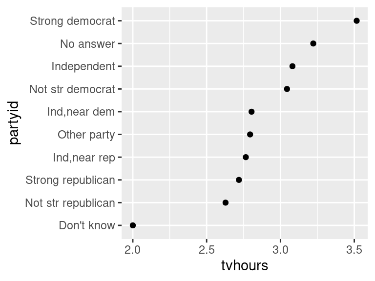
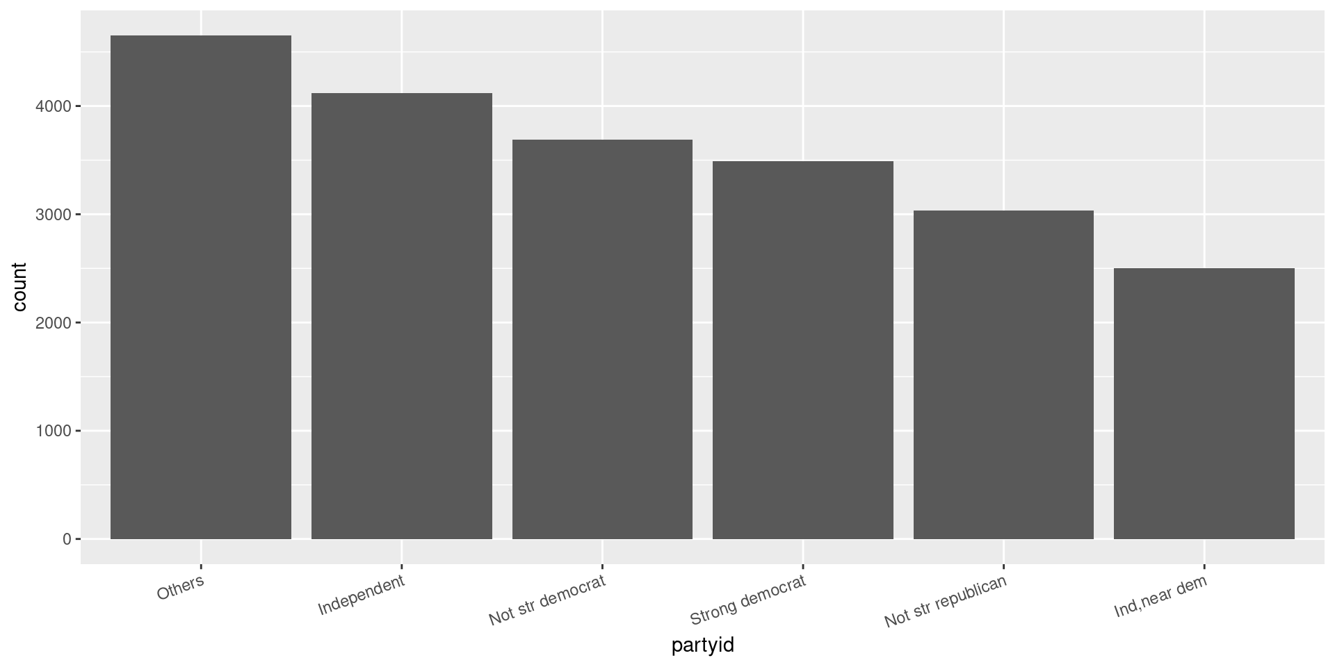
How could we improve the partyid labels?

fct_recode()

• Plot
• Code

gss_cat %>%
  drop_na(tvhours) %>%
  select(partyid, tvhours) %>%
    mutate(partyid = fct_recode(partyid,
    "Republican, strong"    = "Strong republican",
    "Republican, weak"      = "Not str republican",
    "Independent, near rep" = "Ind,near rep",
    "Independent, near dem" = "Ind,near dem",
    "Democrat, weak"        = "Not str democrat",
    "Democrat, strong"      = "Strong democrat")) %>% 
  group_by(partyid) %>%
  summarize(tvhours = mean(tvhours)) %>%
  ggplot(aes(tvhours, fct_reorder(partyid, tvhours))) +
  geom_point() + 
  labs(y = "partyid")

fct_collapse()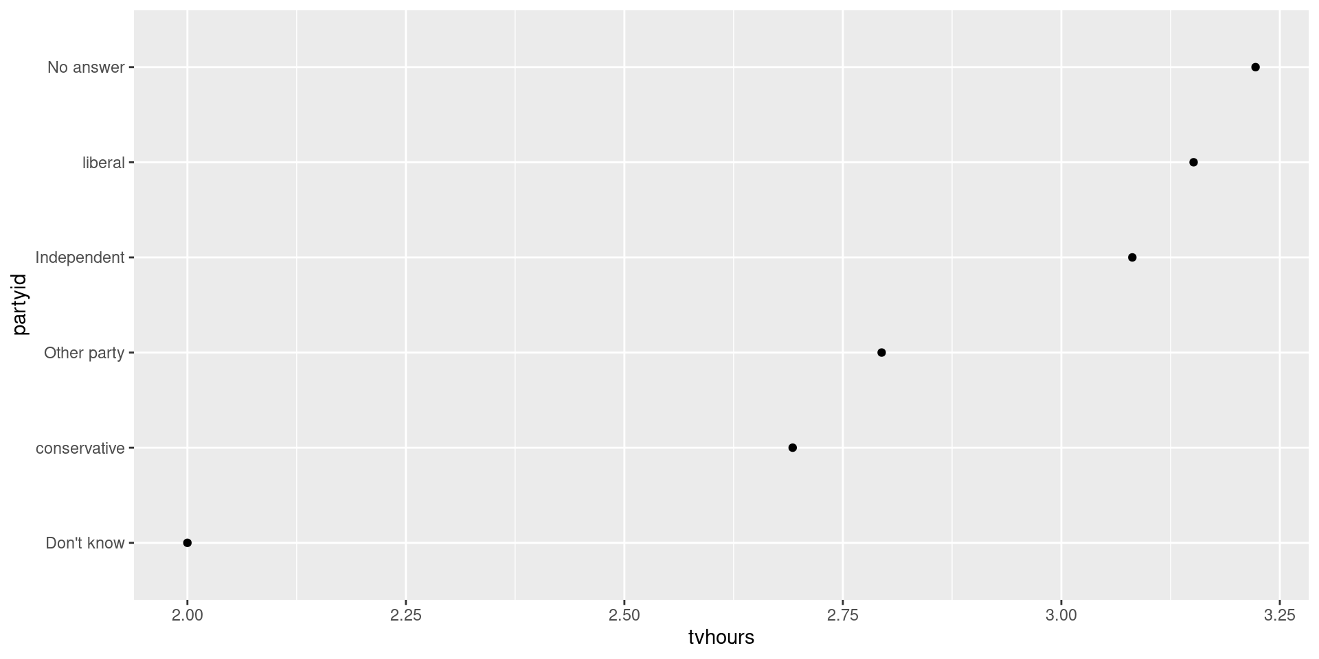

• Plot
• Code

gss_cat %>%
  drop_na(tvhours) %>%
  select(partyid, tvhours) %>%
  mutate(
    partyid = 
      fct_collapse(
        partyid,
        conservative = c("Strong republican", 
                         "Not str republican", 
                         "Ind,near rep"),
        liberal = c("Strong democrat", 
                    "Not str democrat", 
                    "Ind,near dem"))
  ) %>% 
  group_by(partyid) %>%
  summarize(tvhours = mean(tvhours)) %>%
  ggplot(aes(tvhours, fct_reorder(partyid, tvhours))) +
  geom_point() + 
  labs(y = "partyid")

fct_lump()

• Code
• Plot

gss_cat %>%
  mutate(partyid = partyid) %>% 
  mutate(partyid = fct_lump(partyid, n = 5, other_level = "Others")) %>% 
  ggplot(aes(x = fct_infreq(partyid))) + 
  geom_bar() +
  theme(axis.text.x = element_text(angle = 20, 
                                  vjust = 1,
                                  hjust=1)) +
  labs(x = "partyid")

Summary

To enhance your data analysis, you can use the following factor manipulation techniques:

• Reorder the levels to arrange them in a meaningful order.
• Recode the levels to modify the labels or merge similar categories.
• Collapse levels to group multiple categories into one.
• Lump levels to reduce the number of categories by combining less frequent ones.

 Group Activity 2

• Please do the remaining problems in the class activity.
• Submit to Gradescope on moodle when done!

10:00