Basic String Manipulation
STAT 220
Let’s Define Strings
- A string is any sequence of characters
- Define a string by surrounding text with either single quotes or double quotes.
The cat() or writeLines() function displays a string as it is represented inside R.
String Parsing
Definition: pulling apart some text or string to do something with it
The most common tasks in string processing include:
- extracting numbers from strings, e.g. “12%”
- removing unwanted characters from text, e.g. “New Jersey_*”
- finding and replacing characters, e.g. “2,150”
- extracting specific parts of strings, e.g. “Learning #datascience is fun!”
- splitting strings into multiple values, e.g. “123 Main St, Springfield, MA, 01101”
Regular expressions: Regex
Regular expressions are a language for expressing patterns in strings
- Regex can include special characters unlike a regular string
- To use regex in R, you need to use the stringr package
stringr package
- detecting, locating, extracting and replacing elements of strings.
- begin with
str_and take the string as the first argument

stringr cheatsheet
Special characters
Combining strings
Combining strings
str_length()
tells you how many characters are in each entry of a character vector
str_count()
counts the number of non-overlapping matches of a pattern in each entry of a character vector
str_glue()
allows one to interpolate strings and values that have been assigned to names in R
str_sub()
Extract and replace substrings from a character vector
Group Activity 1

- Please clone the
ca11-yourusernamerepository from Github - Please complete problem 1 in today’s class activity.
15:00
More Special Characters
- The | symbol inside a regex means
"or" - The [abe] means one of a,b, or e
- Use
\\nto match a newline character - Use
\\sto match white space characters (spaces, tabs, and newlines) - Use
\\wto match alphanumeric characters (letters and numbers)- can also use
[:alnum:]
- can also use
- Use
\\dto represent digits (numbers)- can also use
[:digit:]
- can also use
Click here for extensive lists
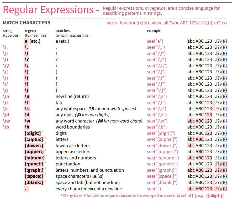
stringr cheatsheet
More Special Characters
^= start of a string$= end of a string.= any character
Quantifiers
*= matches the preceding character any number of times+= matches the preceding character once?= matches the preceding character at most once (i.e. optionally)- {n} = matches the preceding character exactly n times
Try more regexes here
Finding strings
[1] FALSE FALSE FALSE FALSE FALSE FALSE TRUEstr_extract()
Extract just the part of the string matching the specified regex instead of the entire entry
Click for Hint
Extracts the first word from each string in the given vectorstr_split()
splits a string into a list or matrix of pieces based on a supplied pattern
str_replace()
Replaces the first instance of the detected pattern with a specified string.
str_replace_all()
# A tibble: 51 × 4
   state                population total murder_rate
   <chr>                <chr>      <chr>       <dbl>
 1 Alabama              4,853,875  348           7.2
 2 Alaska               737,709    59            8
 3 Arizona              6,817,565  309           4.5
 4 Arkansas             2,977,853  181           6.1
 5 California           38,993,940 1,861         4.8
 6 Colorado             5,448,819  176           3.2
 7 Connecticut          3,584,730  117           3.3
 8 Delaware             944,076    63            6.7
 9 District of Columbia 670,377    162          24.2
10 Florida              20,244,914 1,041         5.1
# ℹ 41 more rows
str_replace_all()
murders %>%
  mutate(population = str_replace_all(population, ",", ""),
         total = str_replace_all(total, ",", ""))
# A tibble: 51 × 4
state population total murder_rate
<chr> <chr> <chr> <dbl>
1 Alabama 4853875 348 7.2
2 Alaska 737709 59 8
3 Arizona 6817565 309 4.5
4 Arkansas 2977853 181 6.1
5 California 38993940 1861 4.8
6 Colorado 5448819 176 3.2
7 Connecticut 3584730 117 3.3
8 Delaware 944076 63 6.7
9 District of Columbia 670377 162 24.2
10 Florida 20244914 1041 5.1
# ℹ 41 more rowsstr_replace_all()
murders %>%
  mutate(population = str_replace_all(population, ",", ""),
         total = str_replace_all(total, ",", "")) %>%
  mutate_at(vars(2:3), as.double)
# A tibble: 51 × 4
state population total murder_rate
<chr> <dbl> <dbl> <dbl>
1 Alabama 4853875 348 7.2
2 Alaska 737709 59 8
3 Arizona 6817565 309 4.5
4 Arkansas 2977853 181 6.1
5 California 38993940 1861 4.8
6 Colorado 5448819 176 3.2
7 Connecticut 3584730 117 3.3
8 Delaware 944076 63 6.7
9 District of Columbia 670377 162 24.2
10 Florida 20244914 1041 5.1
# ℹ 41 more rowsGroup Activity 2
- Please do the remaining problems in the class activity.
- Submit to Gradescope on moodle when done!
15:00