Advanced Web Scraping

STAT 220

Bastola

Scrape table

bow(url = "https://usafacts.org/visualizations/covid-vaccine-tracker-states/state/minnesota")

<polite session> https://usafacts.org/visualizations/covid-vaccine-tracker-states/state/minnesota
    User-agent: polite R package
    robots.txt: 4 rules are defined for 1 bots
   Crawl delay: 5 sec
  The path is scrapable for this user-agent

Click here to take a look at the webpage

Scrape table

bow(url = "https://usafacts.org/visualizations/covid-vaccine-tracker-states/state/minnesota") %>%
  scrape()

{html_document}
<html lang="en">
[1] <head>\n<meta http-equiv="Content-Type" content="text/html; charset=UTF-8 ...
[2] <body>\n<div id="root">\n<div class="MuiContainer-root MuiContainer-disab ...

Click here to take a look at the webpage

Scrape table

bow(url = "https://usafacts.org/visualizations/covid-vaccine-tracker-states/state/minnesota") %>%
  scrape() %>% 
  html_elements(css = "table")

{xml_nodeset (1)}
[1] <table class="MuiTable-root jss228" aria-label="sortable data table" aria ...

Click here to take a look at the webpage

Scrape table

bow(url = "https://usafacts.org/visualizations/covid-vaccine-tracker-states/state/minnesota") %>%
  scrape() %>% 
  html_elements(css = "table") %>% 
  html_table()

[[1]]
# A tibble: 51 × 4
   State      % of population with…¹ `% fully vaccinated` % with booster or ad…²
   <chr>      <chr>                  <chr>                <chr>                 
 1 Alabama    64.3%                  52.5%                20.1%                 
 2 Alaska     72%                    64.4%                30.8%                 
 3 Arizona    76.4%                  63.8%                29.4%                 
 4 Arkansas   68.8%                  56.1%                24%                   
 5 California 85.2%                  74.2%                41.5%                 
 6 Colorado   82.2%                  72.4%                40.5%                 
 7 Connectic… >95%*                  81.8%                44.3%                 
 8 Delaware   86.3%                  71.8%                35.4%                 
 9 District … >95%*                  82.1%                37.9%                 
10 Florida    81.4%                  68.6%                29.4%                 
# ℹ 41 more rows
# ℹ abbreviated names: ¹`% of population with at least one dose`,
#   ²`% with booster or additional dose`

Click here to take a look at the webpage

Scrape table

bow(url = "https://usafacts.org/visualizations/covid-vaccine-tracker-states/state/minnesota") %>%
  scrape() %>% 
  html_elements(css = "table") %>% 
  html_table() %>% 
  pluck(1)

# A tibble: 51 × 4
   State      % of population with…¹ `% fully vaccinated` % with booster or ad…²
   <chr>      <chr>                  <chr>                <chr>                 
 1 Alabama    64.3%                  52.5%                20.1%                 
 2 Alaska     72%                    64.4%                30.8%                 
 3 Arizona    76.4%                  63.8%                29.4%                 
 4 Arkansas   68.8%                  56.1%                24%                   
 5 California 85.2%                  74.2%                41.5%                 
 6 Colorado   82.2%                  72.4%                40.5%                 
 7 Connectic… >95%*                  81.8%                44.3%                 
 8 Delaware   86.3%                  71.8%                35.4%                 
 9 District … >95%*                  82.1%                37.9%                 
10 Florida    81.4%                  68.6%                29.4%                 
# ℹ 41 more rows
# ℹ abbreviated names: ¹`% of population with at least one dose`,
#   ²`% with booster or additional dose`

Click here to take a look at the webpage

Scraping multiple tables

all_url <- "https://finance.yahoo.com/screener/predefined/day_gainers?count=25&offset="

Click here to take a look at the webpage

Scraping multiple tables

all_url <- "https://finance.yahoo.com/screener/predefined/day_gainers?count=25&offset="
idx <- seq(0, 1050, by = 25)

Click here to take a look at the webpage

Scraping multiple tables

all_url <- "https://finance.yahoo.com/screener/predefined/day_gainers?count=25&offset="
idx <- seq(0, 1050, by = 25)
read_html(str_glue("{all_url}{idx[1]}"))

{html_document}
<html data-color-theme="light" id="atomic" class="NoJs desktop" lang="en-US">
[1] <head prefix="og: https://ogp.me/ns#">\n<meta http-equiv="Content-Type" c ...
[2] <body>\n<div id="app"><div class="fin-neo neo-green " data-reactroot="">< ...

Click here to take a look at the webpage

Scraping multiple tables

all_url <- "https://finance.yahoo.com/screener/predefined/day_gainers?count=25&offset="
idx <- seq(0, 1050, by = 25)
read_html(str_glue("{all_url}{idx[1]}")) %>% 
  html_table()

[[1]]
# A tibble: 25 × 10
   Symbol Name   `Price (Intraday)` Change `% Change` Volume `Avg Vol (3 month)`
   <chr>  <chr>               <dbl>  <dbl> <chr>      <chr>  <chr>              
 1 TDS    Telep…              19.7    4.38 +28.63%    9.41M  1.156M             
 2 SITM   SiTim…             124.    27.4  +28.29%    840,9… 235,838            
 3 USM    Unite…              46.0    9.96 +27.67%    2.295M 272,445            
 4 ZLAB   Zai L…              21.0    4.44 +26.80%    3.667M 651,411            
 5 ARHS   Arhau…              15.5    2.28 +17.25%    2.718M 1.258M             
 6 DJTWW  Trump…              22.3    2.86 +14.70%    333,1… 408,140            
 7 PLTK   Playt…               8.87   1.12 +14.45%    2.701M 1.102M             
 8 APP    AppLo…              84.7   10.7  +14.45%    15.11… 4.611M             
 9 UPST   Upsta…              26.2    3.06 +13.24%    10.21… 5.638M             
10 GME    GameS…              18.0    2.09 +13.13%    24.82… 6.537M             
# ℹ 15 more rows
# ℹ 3 more variables: `Market Cap` <chr>, `PE Ratio (TTM)` <chr>,
#   `52 Week Range` <lgl>

Click here to take a look at the webpage

Scraping multiple tables

all_url <- "https://finance.yahoo.com/screener/predefined/day_gainers?count=25&offset="
idx <- seq(0, 1050, by = 25)
read_html(str_glue("{all_url}{idx[1]}")) %>% 
  html_table() %>% 
  purrr::pluck(1)

# A tibble: 25 × 10
   Symbol Name   `Price (Intraday)` Change `% Change` Volume `Avg Vol (3 month)`
   <chr>  <chr>               <dbl>  <dbl> <chr>      <chr>  <chr>              
 1 TDS    Telep…              19.7    4.38 +28.63%    9.41M  1.156M             
 2 SITM   SiTim…             124.    27.4  +28.29%    840,9… 235,838            
 3 USM    Unite…              46.0    9.96 +27.67%    2.295M 272,445            
 4 ZLAB   Zai L…              21.0    4.44 +26.80%    3.667M 651,411            
 5 ARHS   Arhau…              15.5    2.28 +17.25%    2.718M 1.258M             
 6 DJTWW  Trump…              22.3    2.86 +14.70%    333,1… 408,140            
 7 PLTK   Playt…               8.87   1.12 +14.45%    2.701M 1.102M             
 8 APP    AppLo…              84.7   10.7  +14.45%    15.11… 4.611M             
 9 UPST   Upsta…              26.2    3.06 +13.24%    10.21… 5.638M             
10 GME    GameS…              18.0    2.09 +13.13%    24.82… 6.537M             
# ℹ 15 more rows
# ℹ 3 more variables: `Market Cap` <chr>, `PE Ratio (TTM)` <chr>,
#   `52 Week Range` <lgl>

Click here to take a look at the webpage

Scraping multiple tables

all_url <- "https://finance.yahoo.com/screener/predefined/day_gainers?count=25&offset="
idx <- seq(0, 1050, by = 25)
read_html(str_glue("{all_url}{idx[1]}")) %>% 
  html_table() %>% 
  purrr::pluck(1) %>% 
  janitor::clean_names()

# A tibble: 25 × 10
   symbol name       price_intraday change percent_change volume avg_vol_3_month
   <chr>  <chr>               <dbl>  <dbl> <chr>          <chr>  <chr>          
 1 TDS    Telephone…          19.7    4.38 +28.63%        9.41M  1.156M         
 2 SITM   SiTime Co…         124.    27.4  +28.29%        840,9… 235,838        
 3 USM    United St…          46.0    9.96 +27.67%        2.295M 272,445        
 4 ZLAB   Zai Lab L…          21.0    4.44 +26.80%        3.667M 651,411        
 5 ARHS   Arhaus, I…          15.5    2.28 +17.25%        2.718M 1.258M         
 6 DJTWW  Trump Med…          22.3    2.86 +14.70%        333,1… 408,140        
 7 PLTK   Playtika …           8.87   1.12 +14.45%        2.701M 1.102M         
 8 APP    AppLovin …          84.7   10.7  +14.45%        15.11… 4.611M         
 9 UPST   Upstart H…          26.2    3.06 +13.24%        10.21… 5.638M         
10 GME    GameStop …          18.0    2.09 +13.13%        24.82… 6.537M         
# ℹ 15 more rows
# ℹ 3 more variables: market_cap <chr>, pe_ratio_ttm <chr>,
#   x52_week_range <lgl>

Click here to take a look at the webpage

Scraping multiple tables

all_url <- "https://finance.yahoo.com/screener/predefined/day_gainers?count=25&offset="
idx <- seq(0, 1050, by = 25)
read_html(str_glue("{all_url}{idx[1]}")) %>% 
  html_table() %>% 
  purrr::pluck(1) %>% 
  janitor::clean_names() %>% 
  mutate(across(everything(), as.character)) # for consistent data joins

# A tibble: 25 × 10
   symbol name       price_intraday change percent_change volume avg_vol_3_month
   <chr>  <chr>      <chr>          <chr>  <chr>          <chr>  <chr>          
 1 TDS    Telephone… 19.68          4.38   +28.63%        9.41M  1.156M         
 2 SITM   SiTime Co… 124.34         27.42  +28.29%        840,9… 235,838        
 3 USM    United St… 45.95          9.96   +27.67%        2.295M 272,445        
 4 ZLAB   Zai Lab L… 21.01          4.44   +26.80%        3.667M 651,411        
 5 ARHS   Arhaus, I… 15.5           2.28   +17.25%        2.718M 1.258M         
 6 DJTWW  Trump Med… 22.32          2.86   +14.70%        333,1… 408,140        
 7 PLTK   Playtika … 8.87           1.12   +14.45%        2.701M 1.102M         
 8 APP    AppLovin … 84.69          10.69  +14.45%        15.11… 4.611M         
 9 UPST   Upstart H… 26.17          3.06   +13.24%        10.21… 5.638M         
10 GME    GameStop … 18.01          2.09   +13.13%        24.82… 6.537M         
# ℹ 15 more rows
# ℹ 3 more variables: market_cap <chr>, pe_ratio_ttm <chr>,
#   x52_week_range <chr>

Click here to take a look at the webpage

Code
Data

all_url <- "https://finance.yahoo.com/screener/predefined/day_gainers?count=25&offset="
idx <- seq(0, 1050, by = 25)

my_df <- map_df(idx, ~ {
  new_webpage <- read_html(str_glue("{all_url}{.x}")) 
  table_new <- html_table(new_webpage)[[1]] %>%
    janitor::clean_names() %>% 
    mutate(across(everything(), as.character))
  return(table_new)
})

Please clone the ca17-yourusername repository from Github
Please do the problem 1 in the class activity for today

10:00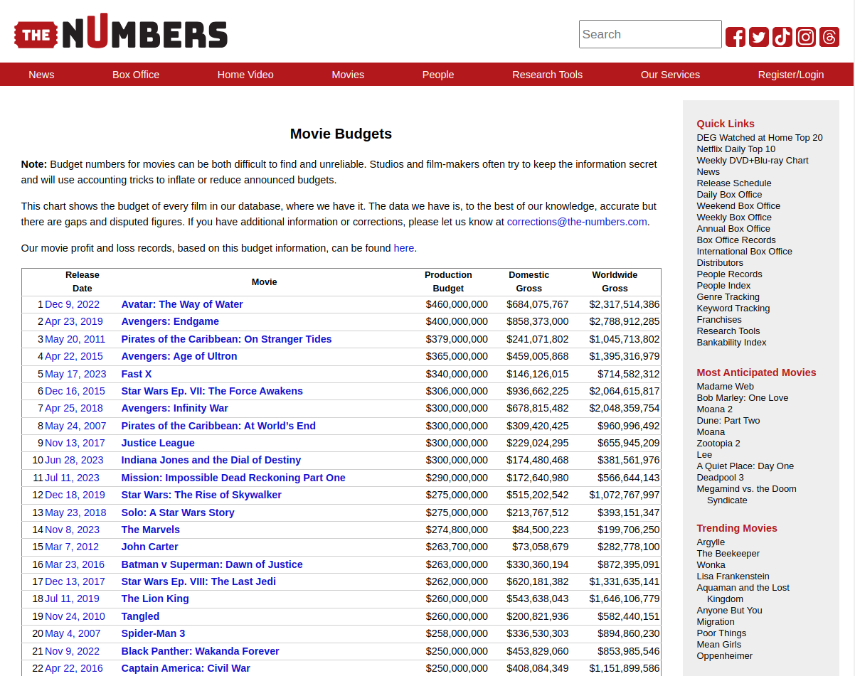

{width = “80%}

Scrape, Tidy, and Visualize

df_movies %>% 
mutate(
  ID = row_number(), 
  ProductionBudget = parse_number(ProductionBudget),
  DomesticGross = parse_number(DomesticGross),
  WorldwideGross = parse_number(WorldwideGross),
  ReleaseDate = mdy(ReleaseDate),
  MonthOfRelease = month(ReleaseDate, label = TRUE, abbr = TRUE),
  YearOfRelease = year(ReleaseDate)
) %>%
replace_na(list(ReleaseDate = make_date(year = 1900))) %>%
  group_by(MonthOfRelease) %>%
  summarize(AverageByMonth = mean(DomesticGross, na.rm = TRUE)) -> 
  df_DomesticGross_month

Plot
Code

library(plotly)
fig <- df_DomesticGross_month %>% 
  plot_ly(labels = ~MonthOfRelease, values = ~AverageByMonth)
fig <- fig %>% add_pie(hole = 0.6)
fig <- fig %>% layout(title = "Average Domestic Gross by Month",  
                      showlegend = F,
                      xaxis = list(showgrid = FALSE, 
                                   zeroline = FALSE, 
                                   showticklabels = FALSE),
                      yaxis = list(showgrid = FALSE, 
                                   zeroline = FALSE, 
                                   showticklabels = FALSE))

fig

DT: Interactive Data Tables

library(ggplot2movies)
library(DT)
movies %>% select(1:6) %>% tidyr::drop_na(budget) %>% 
  filter(rating > 8, votes > 1000) %>% 
  datatable(fillContainer = FALSE,  options = list(pageLength = 6, scrollY = '400px'))

Advanced Web Scraping

Scrape table

Scrape table

Scrape table

Scrape table

Scrape table

Scraping multiple tables

Scraping multiple tables

Scraping multiple tables

Scraping multiple tables

Scraping multiple tables

Scraping multiple tables

Scraping multiple tables

Group Activity 1

Scrape, Tidy, and Visualize

DT: Interactive Data Tables