Intro to Classification
STAT 220
Classification
Predicting what category a (future) observation falls into
- Astronomy: Whether an exoplanet is habitable (or not)
- Filtering: Identify spam emails
- Medicine: Use lab results to determine who has a disease (or not)
- Product preference: make product recommendations based on past purchases
Fire can be deadly, destroying homes, wildlife habitat and timber, and polluting the air with harmful emissions.Predicting the next forest fire ..
Dataset
- contains a culmination of forest fire observations
- based on two regions of Algeria: the Bejaia region and the Sidi Bel-Abbes region.
- from June 2012 to September 2012
Click here to learn more about the dataset
Data Description
| Variable | Description |
|---|---|
Date |
(DD-MM-YYYY) Day, month, year |
Temp |
Noon temperature in Celsius degrees: 22 to 42 |
RH |
Relative Humidity in percentage: 21 to 90 |
Ws |
Wind speed in km/h: 6 to 29 |
Rain |
Daily total rain in mm: 0 to 16.8 |
Fine Fuel Moisture Code (FFMC) index |
28.6 to 92.5 |
Duff Moisture Code (DMC) index |
1.1 to 65.9 |
Drought Code (DC) index |
7 to 220.4 |
Initial Spread Index (ISI) index |
0 to 18.5 |
Buildup Index (BUI) index |
1.1 to 68 |
Fire Weather Index (FWI) index |
0 to 31.1 |
Classes |
Two classes, namely fire and not fire |
Glimpse of the data
| date | temperature | rh | ws | rain | ffmc | dmc | dc | isi | bui | fwi | classes |
|---|---|---|---|---|---|---|---|---|---|---|---|
| 2012-06-01 | 29 | 57 | 18 | 0.0 | 65.7 | 3.4 | 7.6 | 1.3 | 3.4 | 0.5 | not fire |
| 2012-06-02 | 29 | 61 | 13 | 1.3 | 64.4 | 4.1 | 7.6 | 1.0 | 3.9 | 0.4 | not fire |
| 2012-06-03 | 26 | 82 | 22 | 13.1 | 47.1 | 2.5 | 7.1 | 0.3 | 2.7 | 0.1 | not fire |
| 2012-06-04 | 25 | 89 | 13 | 2.5 | 28.6 | 1.3 | 6.9 | 0.0 | 1.7 | 0.0 | not fire |
| 2012-06-05 | 27 | 77 | 16 | 0.0 | 64.8 | 3.0 | 14.2 | 1.2 | 3.9 | 0.5 | not fire |
| 2012-06-06 | 31 | 67 | 14 | 0.0 | 82.6 | 5.8 | 22.2 | 3.1 | 7.0 | 2.5 | fire |
| 2012-06-07 | 33 | 54 | 13 | 0.0 | 88.2 | 9.9 | 30.5 | 6.4 | 10.9 | 7.2 | fire |
| 2012-06-08 | 30 | 73 | 15 | 0.0 | 86.6 | 12.1 | 38.3 | 5.6 | 13.5 | 7.1 | fire |
| 2012-06-09 | 25 | 88 | 13 | 0.2 | 52.9 | 7.9 | 38.8 | 0.4 | 10.5 | 0.3 | not fire |
| 2012-06-10 | 28 | 79 | 12 | 0.0 | 73.2 | 9.5 | 46.3 | 1.3 | 12.6 | 0.9 | not fire |
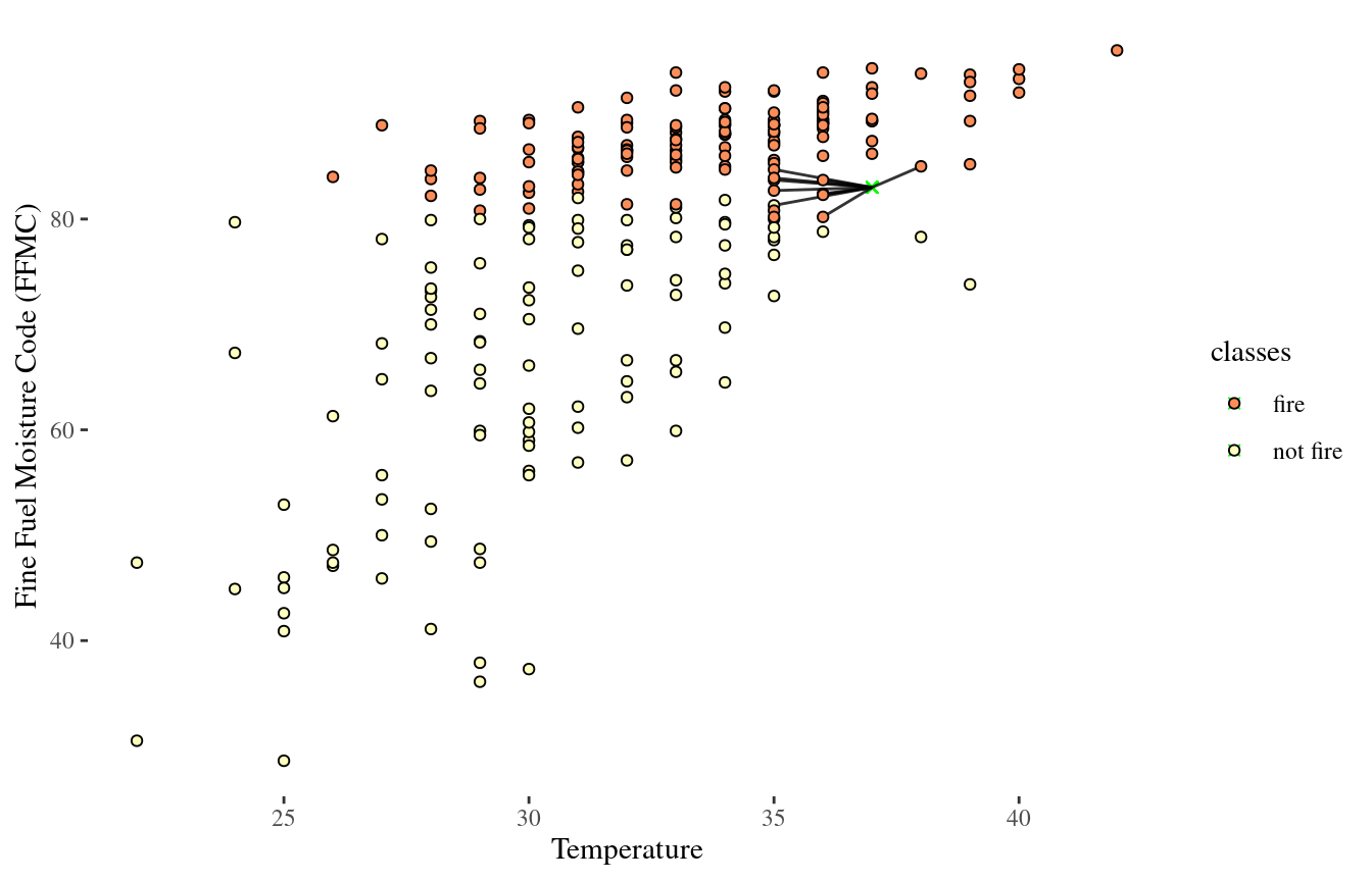
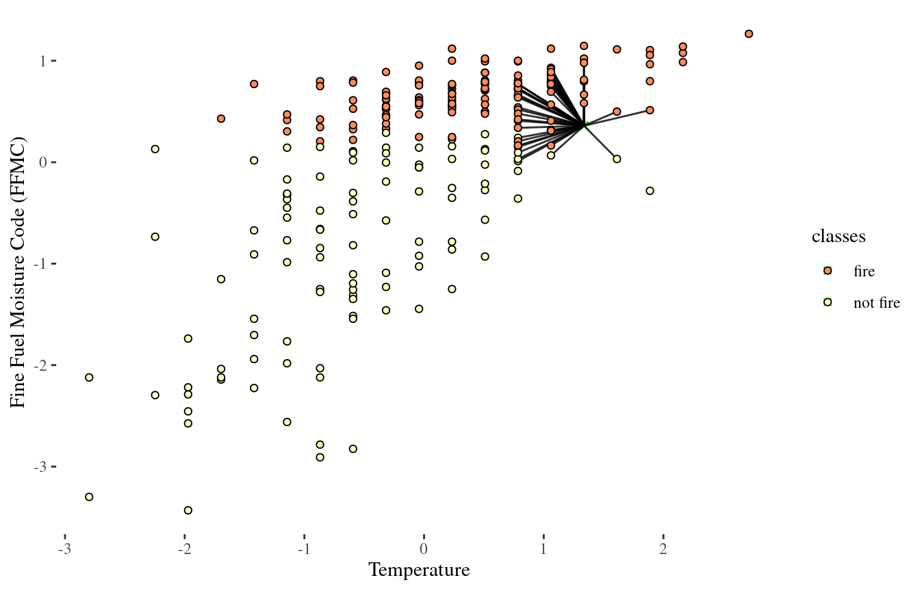
Scatterplot
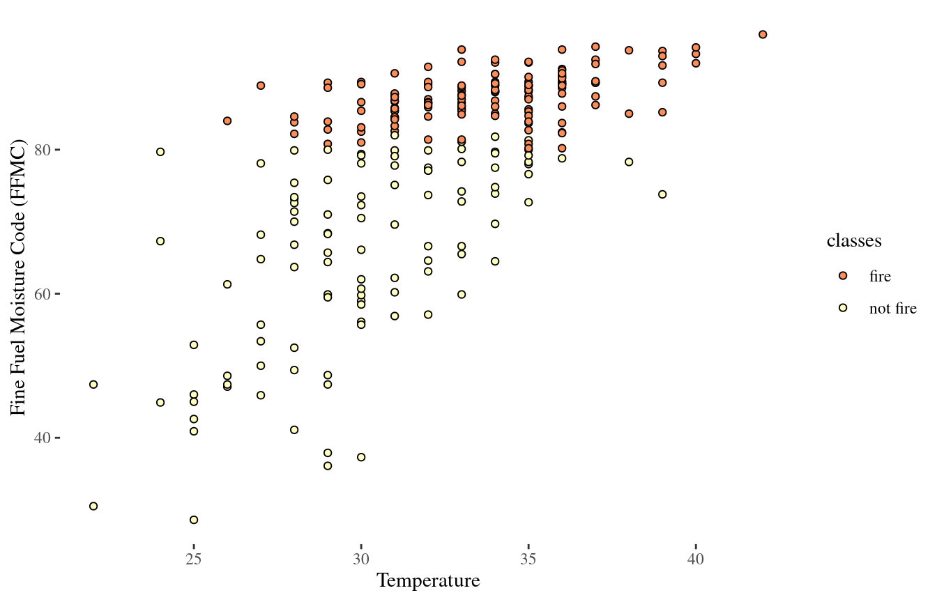
Classifying a new observation?
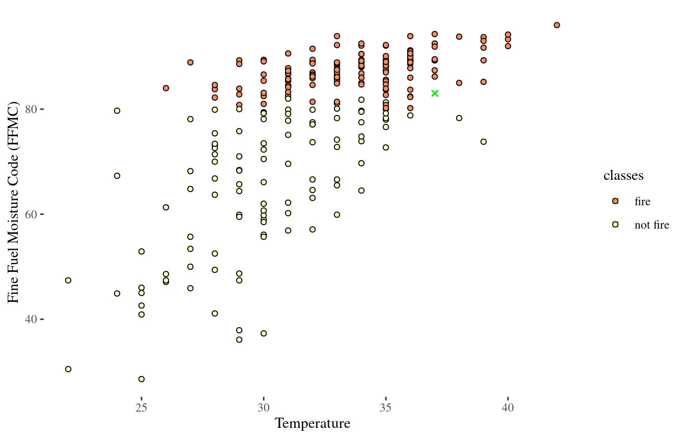
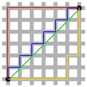
Euclidean distance: the straight line distance between two points on the x-y plane with coordinates
\((x_a, y_a)\) and \((x_b,y_b)\)
\[{\rm Distance} = \sqrt{\left(x_a - x_b \right)^2 + \left( y_a - y_b \right)^2}\]
Manhattan distance: the “taxi-cab” distance between two points on the x-y plane
\[{\rm Distance} = \left|x_a - x_b \right| + \left| y_a - y_b \right|\]
Looking at Euclidean distance
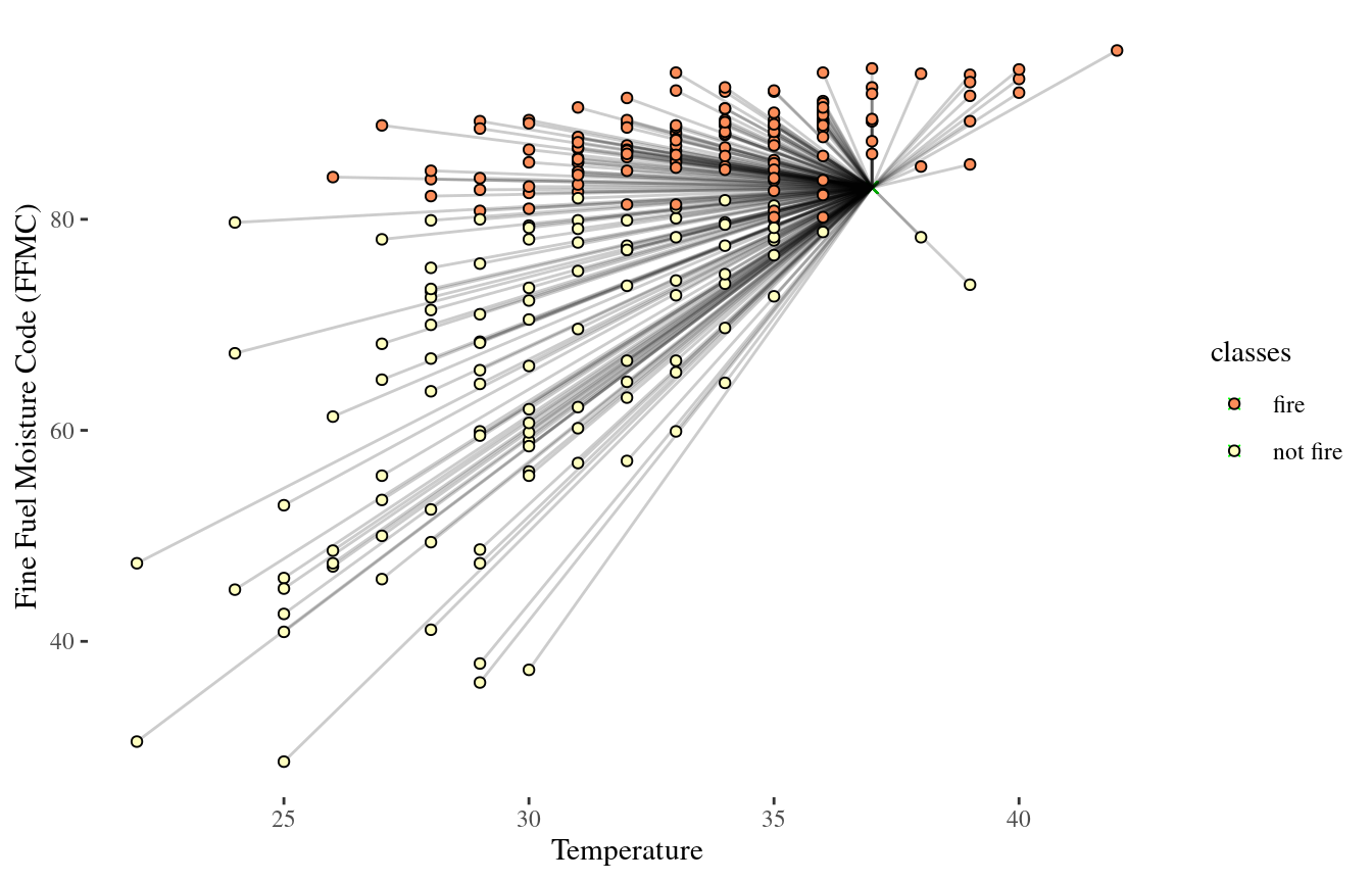
1-Nearest Neighbor (NN)

10-NN

10-NN
Wait, something is not quite right..
Need to standardize data
- Predictors with larger variation will have larger influence on which cases are “nearest” neighbors
- Methods relying on distance can be sensitive (i.e. not invariant) to the scale of the predictors
- Standardizing only shifts and rescales the variable, it doesn’t change the shape of the distribution
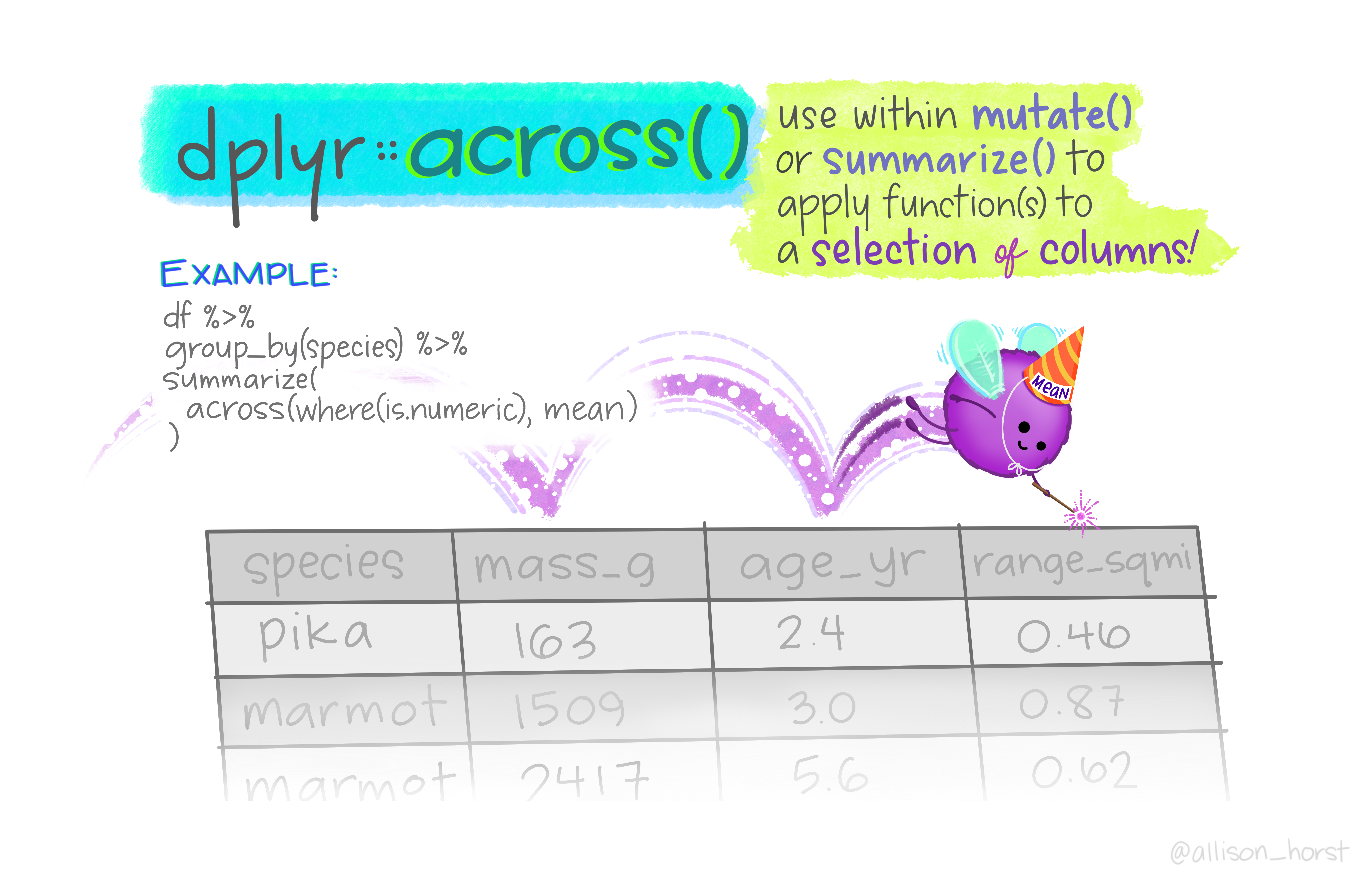
Standardized data
fire1 <- fire %>% mutate(across(where(is.numeric), standardize))
fire1 %>% head() %>% knitr::kable()| date | temperature | rh | ws | rain | ffmc | dmc | dc | isi | bui | fwi | classes |
|---|---|---|---|---|---|---|---|---|---|---|---|
| 2012-06-01 | -0.8688614 | -0.3399715 | 0.8914370 | -0.3808708 | -0.8461805 | -0.9102414 | -0.8775901 | -0.8286454 | -0.9340836 | -0.8783457 | not fire |
| 2012-06-02 | -0.8688614 | -0.0702145 | -0.8870457 | 0.2680887 | -0.9367751 | -0.8537581 | -0.8775901 | -0.9008609 | -0.8989427 | -0.8917856 | not fire |
| 2012-06-03 | -1.6957543 | 1.3460097 | 2.3142231 | 6.1586438 | -2.1423802 | -0.9828629 | -0.8880798 | -1.0693637 | -0.9832809 | -0.9321051 | not fire |
| 2012-06-04 | -1.9713852 | 1.8180845 | -0.8870457 | 0.8671282 | -3.4316110 | -1.0796914 | -0.8922757 | -1.1415792 | -1.0535628 | -0.9455449 | not fire |
| 2012-06-05 | -1.4201233 | 1.0088135 | 0.1800439 | -0.3808708 | -0.9088999 | -0.9425176 | -0.7391255 | -0.8527172 | -0.8989427 | -0.8783457 | not fire |
| 2012-06-06 | -0.3175995 | 0.3344210 | -0.5313491 | -0.3808708 | 0.3315493 | -0.7165844 | -0.5712896 | -0.3953525 | -0.6810689 | -0.6095490 | fire |
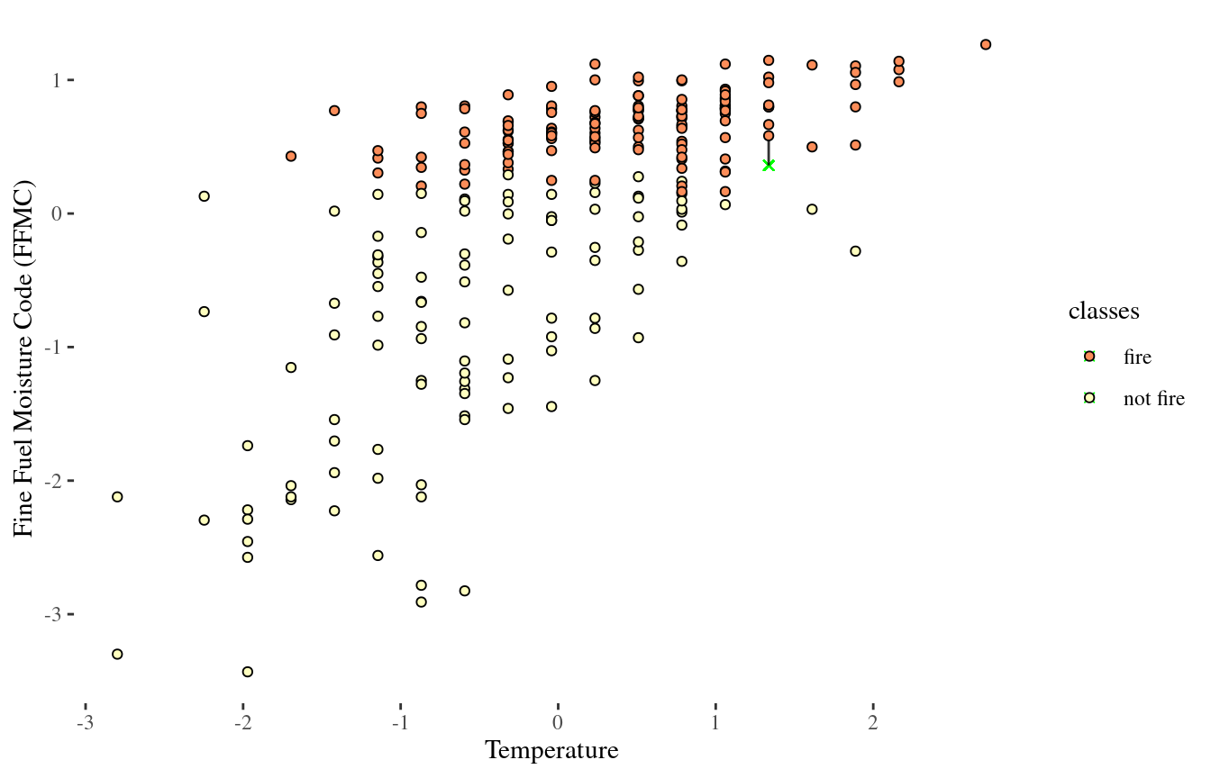
1-NN again
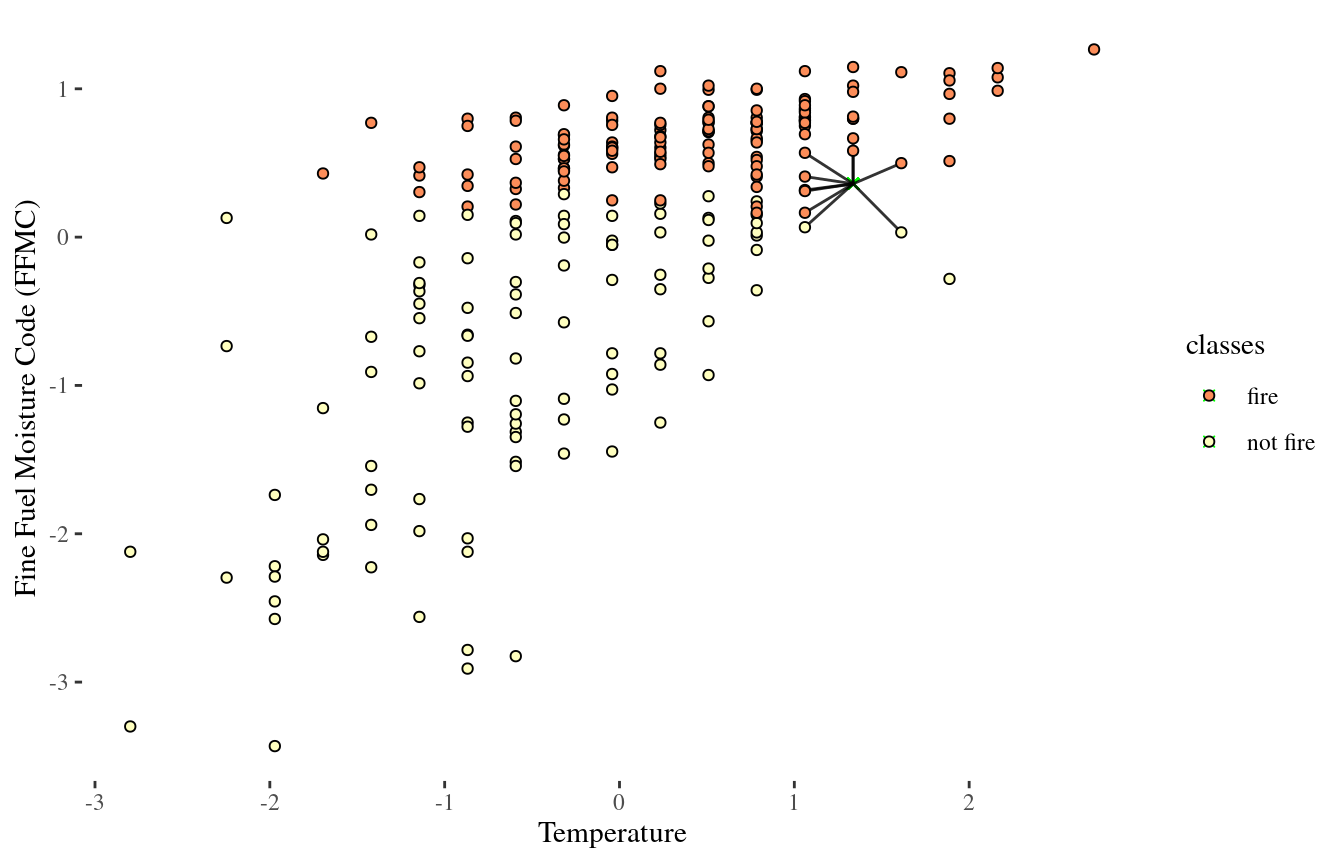
10-NN again
50-NN again
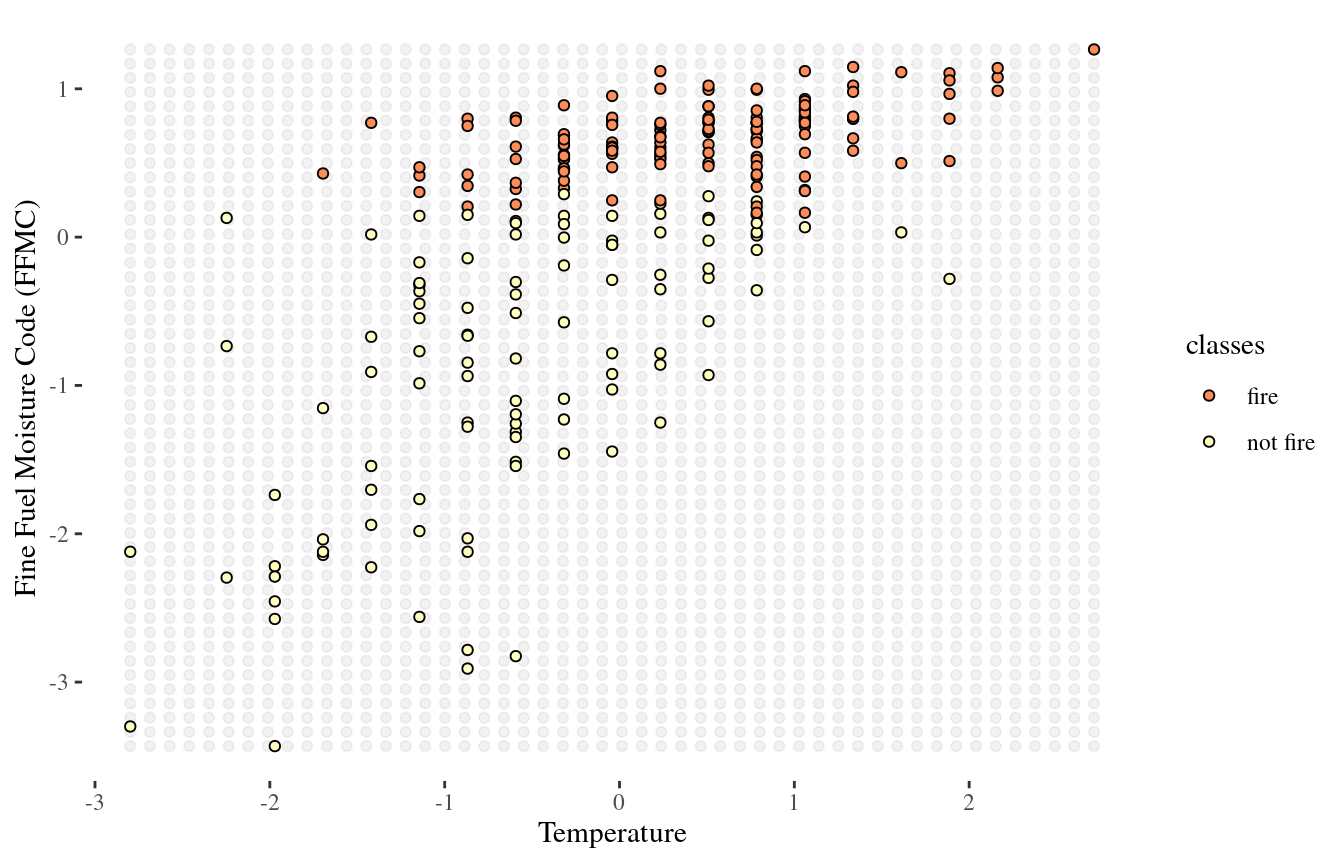
Visualizing the decision boundary
We can map out the region in feature-space where the classifier would predict ‘fire’, and the kinds where it would predict ‘not fire’
There is some boundary between the two, where points on one side of the boundary will be classified ‘fire’ and points on the other side will be classified ‘not fire’
This boundary is called decision boundary
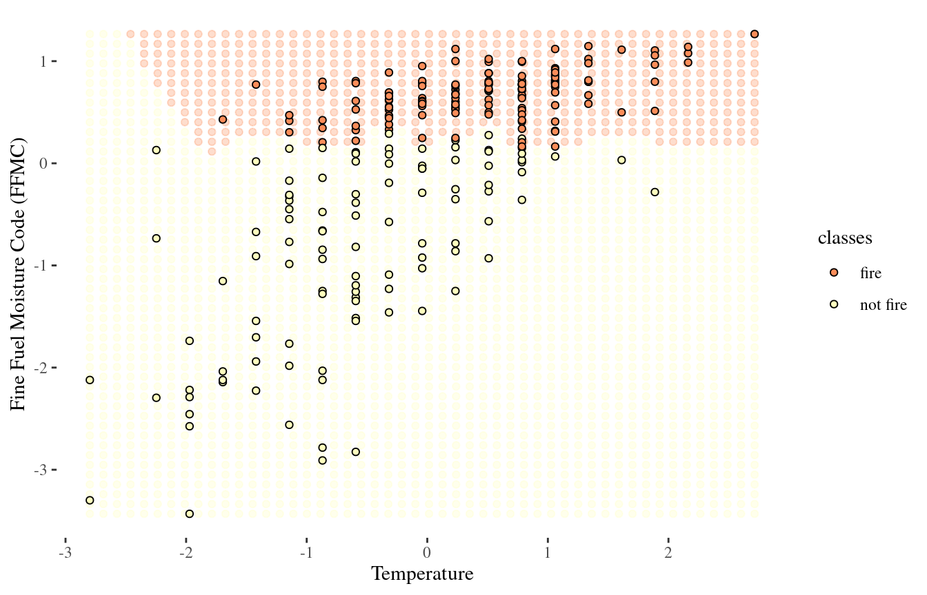
Visualizing the decision boundary
1-NN decision boundary
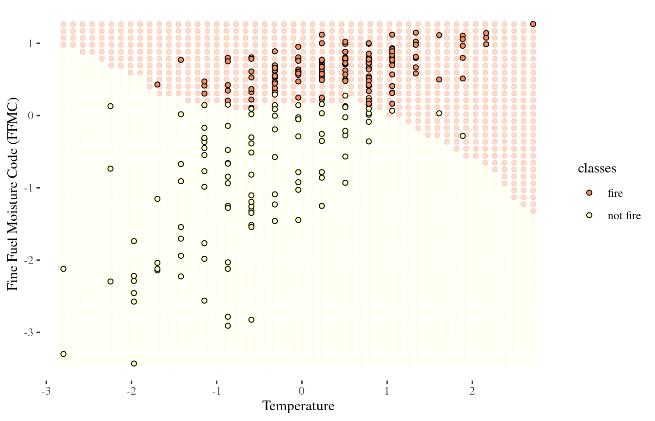
25-NN decision boundary

a collection of packages for modeling and machine learning using tidyverse principles
1. Load data and convert to correct data types
fire_raw <- read_csv("https://raw.githubusercontent.com/deepbas/statdatasets/main/Algeriafires.csv") %>%
  janitor::clean_names() %>% tidyr::drop_na() %>%
  mutate(classes = factor(classes)) %>%
  mutate_at(c(10,13), as.numeric) %>%
  select(temperature, ffmc, classes)
head(fire_raw)
# A tibble: 6 × 3
temperature ffmc classes
<dbl> <dbl> <fct>
1 29 65.7 not fire
2 29 64.4 not fire
3 26 47.1 not fire
4 25 28.6 not fire
5 27 64.8 not fire
6 31 82.6 fire 
2. Create a recipe for data preprocessing
3. Apply the recipe to the data set
# A tibble: 243 × 3
   temperature   ffmc classes
         <dbl>  <dbl> <fct>
 1      -0.869 -0.846 not fire
 2      -0.869 -0.937 not fire
 3      -1.70  -2.14  not fire
 4      -1.97  -3.43  not fire
 5      -1.42  -0.909 not fire
 6      -0.318  0.332 fire
 7       0.234  0.722 fire
 8      -0.593  0.610 fire
 9      -1.97  -1.74  not fire
10      -1.14  -0.324 not fire
# ℹ 233 more rows
4. Create a model specification
5. Fit the model on the preprocessed data
6. Classify
Suppose we get two new observations, use predict to classify the observations
Further Practice: Pima Indians Diabetes
- Owned by the National Institute of Diabetes and Digestive and Kidney Diseases
- A data frame with 768 observations on 9 variables.
- We have the lab results of 158 patients, including whether they have CKD
- Response variable:
diabetes=pos,neg - Predictor variables: pregnant, glucose, pressure, triceps, insulin, mass, pedigree, age
Variables
| Variable | Description |
|---|---|
pregnant |
Number of times pregnant |
glucose |
Plasma glucose concentration (glucose tolerance test) |
pressure |
Diastolic blood pressure (mm Hg) |
triceps |
Triceps skinfold thickness (mm) |
insulin |
2-Hour serum insulin (mu U/ml) |
mass |
Body mass index (weight in kg/(height in m)\²) |
pedigree |
Diabetes pedigree function |
age |
Age (years) |
diabetes |
diabetes case (pos/neg) |
Group Activity 1

- Please clone the
ca21-yourusernamerepository from Github - Please do the problems in the class activity for today
10:00