Model Accuracy and Evaluation

STAT 220

Bastola

Recap: KNN (K- Nearest Neighbor)

• Supervised machine learning algorithm i.e., it requires labeled data for training

• Need to tell the algorithm the exact number of neighbors (K) we want to consider

Training and Testing

Training: Fitting a model with certain hyper-parameters on a particular subset of the dataset

Testing: Test the model on a different subset of the dataset to get an estimate of a final, unbiased assessment of the model’s performance

Workflows

A machine learning workflow (the “black box”) containing model specification and preprocessing recipe/formula

Forest Fire : Data Description

Variable	Description
Date	(DD-MM-YYYY) Day, month, year
Temp	Noon temperature in Celsius degrees: 22 to 42
RH	Relative Humidity in percentage: 21 to 90
Ws	Wind speed in km/h: 6 to 29
Rain	Daily total rain in mm: 0 to 16.8
Fine Fuel Moisture Code (FFMC) index	28.6 to 92.5
Duff Moisture Code (DMC) index	1.1 to 65.9
Drought Code (DC) index	7 to 220.4
Initial Spread Index (ISI) index	0 to 18.5
Buildup Index (BUI) index	1.1 to 68
Fire Weather Index (FWI) index	0 to 31.1
Classes	Two classes, namely .bold[fire] and .bold[not fire]

1. Create a workflow: Split raw data

set.seed(123) # set seed for reproducibility
fire_raw <- fire %>% select(temperature, isi, classes)
# split the data randomly into training and testing set, 75-25
fire_split <- initial_split(fire_raw, prop = 0.75) 

# Create training data
(fire_train <- fire_split %>% training())

# A tibble: 182 × 3
   temperature   isi classes 
         <dbl> <dbl> <chr>   
 1          38   4.1 fire    
 2          34  14.3 fire    
 3          33   6.7 fire    
 4          30   1   not fire
 5          35   7.5 fire    
 6          34   7.3 fire    
 7          33   2.8 fire    
 8          31   2.5 not fire
 9          34   3   not fire
10          33  14.2 fire    
# ℹ 172 more rows

# Create testing data
(fire_test <- fire_split %>% testing())

# A tibble: 61 × 3
   temperature   isi classes 
         <dbl> <dbl> <chr>   
 1          29   1   not fire
 2          26   0.3 not fire
 3          26   4.8 fire    
 4          28   0.4 not fire
 5          31   0.7 not fire
 6          31   2.5 not fire
 7          34   9.2 fire    
 8          32   7.6 fire    
 9          32   2.2 not fire
10          29   1.1 not fire
# ℹ 51 more rows

2. Make a recipe

fire_recipe <- recipe(classes ~ ., data = fire_raw) %>%
  step_scale(all_predictors()) %>% # scale the predictors
  step_center(all_predictors()) # center the predictors

3. Specify the model

fire_knn_spec <- nearest_neighbor(mode = "classification",
                                  engine = "kknn",
                                  weight_func = "rectangular",
                                  neighbors = 5)

4. Define the workflow object

fire_workflow <- workflow() %>% # initialize a workflow
  add_recipe(fire_recipe) %>% # add recipe
  add_model(fire_knn_spec) # add model specification

5. Fit the model

fire_fit <- fit(fire_workflow, data = fire_train)

Fitted workflow

fire_fit

══ Workflow [trained] ══════════════════════════════════════════════════════════
Preprocessor: Recipe
Model: nearest_neighbor()

── Preprocessor ────────────────────────────────────────────────────────────────
2 Recipe Steps

• step_scale()
• step_center()

── Model ───────────────────────────────────────────────────────────────────────

Call:
kknn::train.kknn(formula = ..y ~ ., data = data, ks = min_rows(5,     data, 5), kernel = ~"rectangular")

Type of response variable: nominal
Minimal misclassification: 0.03296703
Best kernel: rectangular
Best k: 5

6. Evaluate the model on test dataset

test_features <- fire_test %>% select(temperature, isi) 
fire_pred <- predict(fire_fit, test_features, type = "raw")
fire_results <- fire_test %>% 
  select(classes) %>% 
  bind_cols(predicted = fire_pred)

7. Compare the known labels and predicted labels

knitr::kable(head(fire_results, 5))

classes	predicted
not fire	not fire
not fire	not fire
fire	fire
not fire	not fire
not fire	not fire

 Group Activity 1

• Please clone the ca22-yourusername repository from Github
• Please do problem 1 in the class activity for today

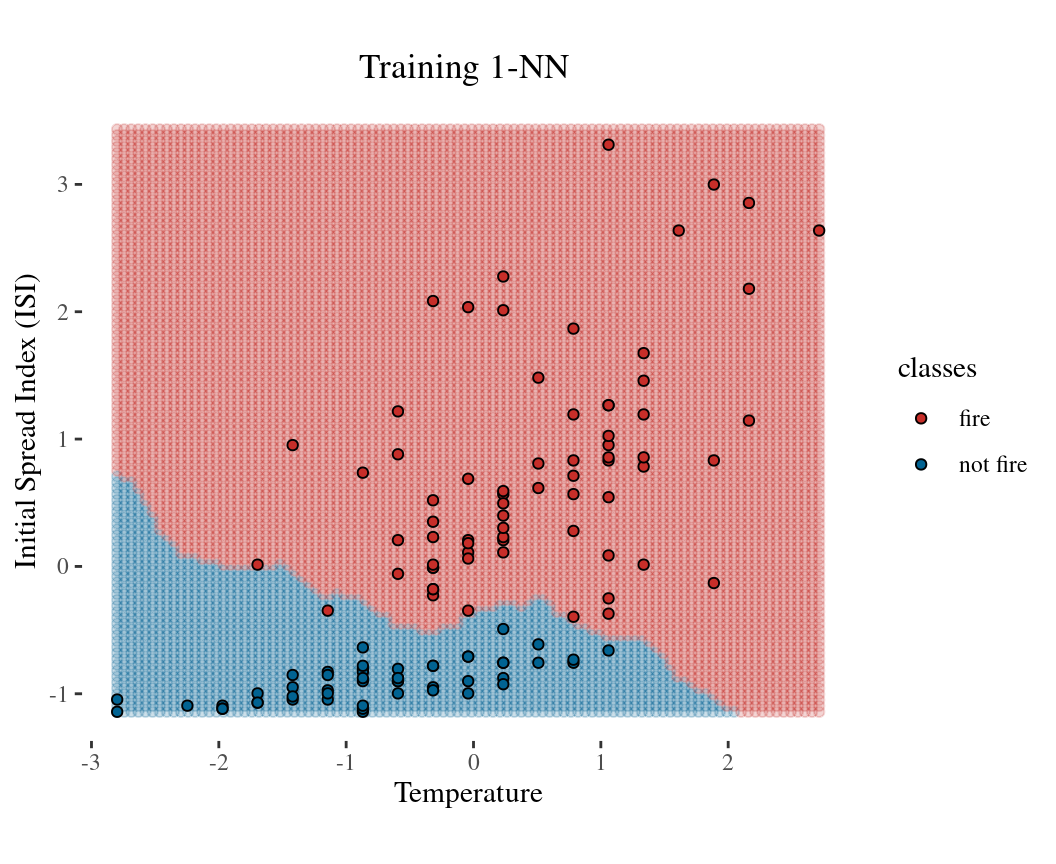
10:00

How to choose the number of neighbors in a principled way?

• Visualizing boundary
• Code
• Take Away

ggplot(data = fire1, aes(x = temperature, y = isi , fill = classes)) +
  geom_point(color = "black", pch = 21) +
  labs(x = "Temperature", y = "Initial Spread Index (ISI)") +
  ggthemes::scale_fill_wsj() +
  theme_tufte()

• We normally don’t have a clear separation between classes and usually have more than 2 features.

• Eyeballing on a plot to discern the classes is not very helpful in the practical sense

Evaluating accuracy

We want to evaluate classifiers based on some accuracy metrics.

• Randomly split data set into two pieces: training set and test set

• Train (i.e. fit) KNN on the training set

• Make predictions on the test set

• See how good those predictions are

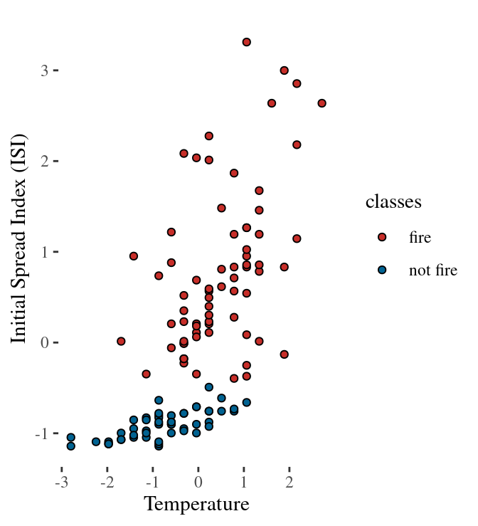
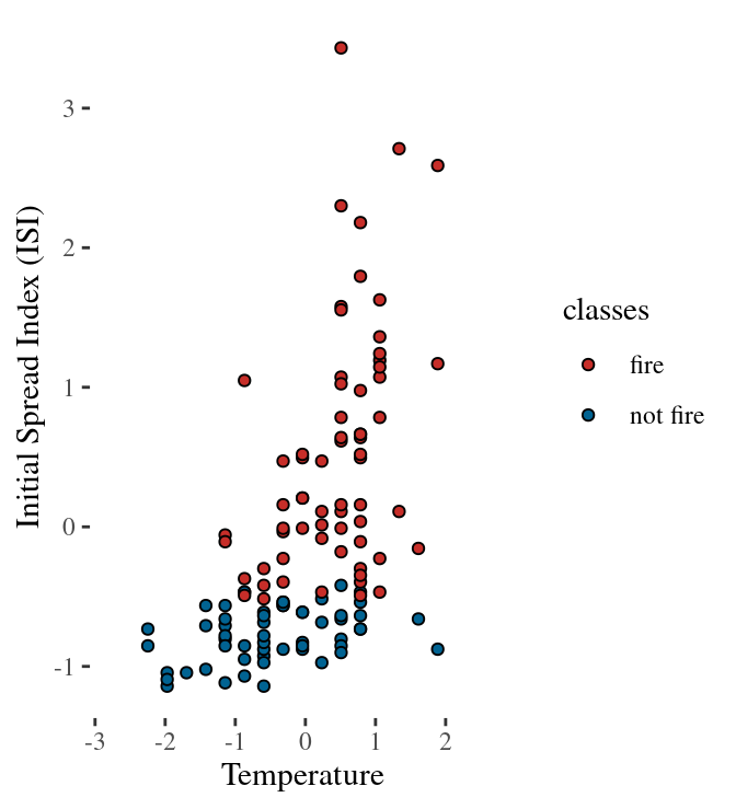
Train (left) and test (right) dataset (50-50)

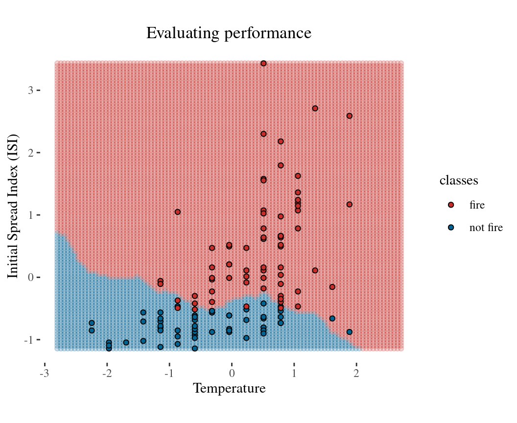
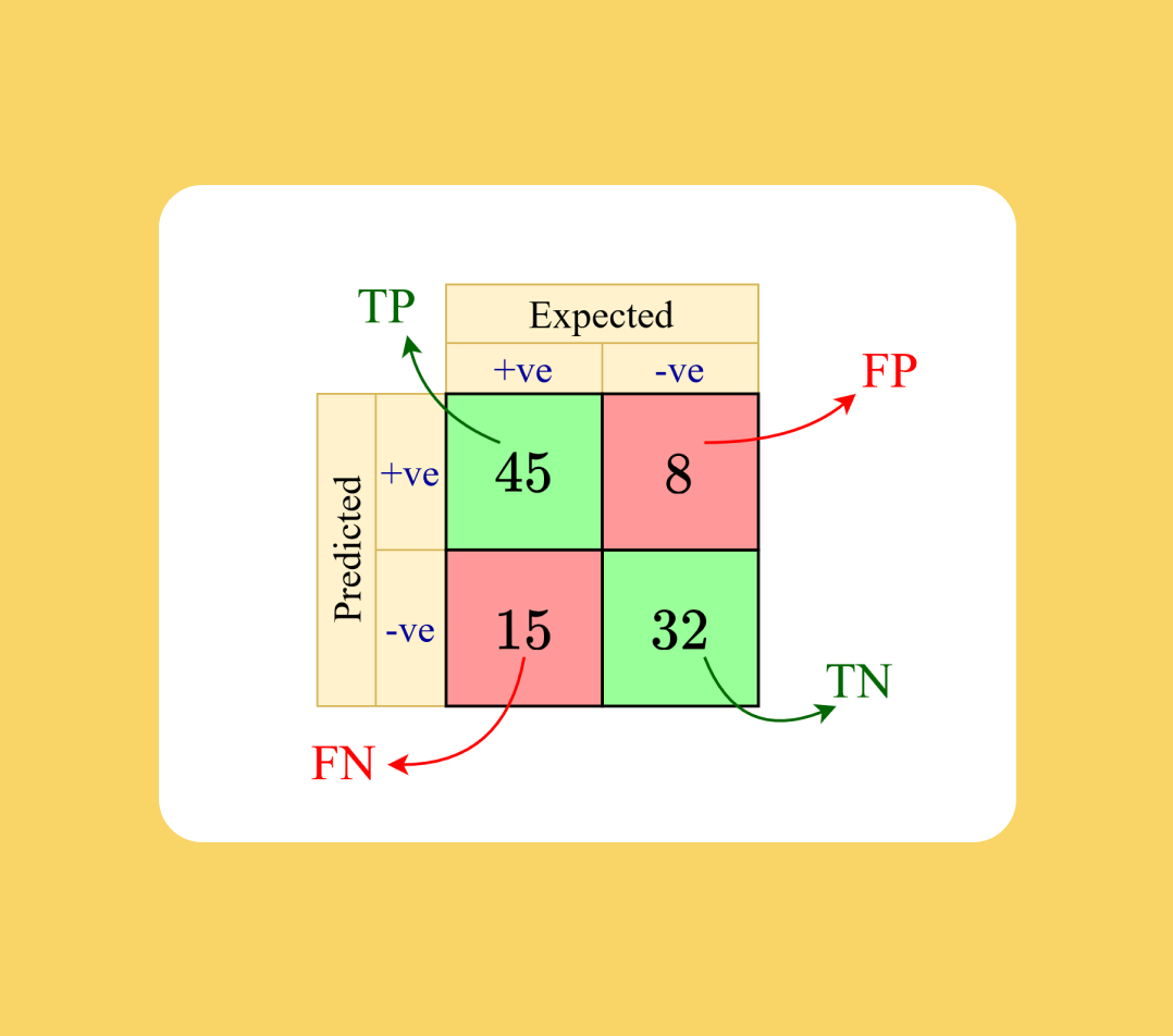
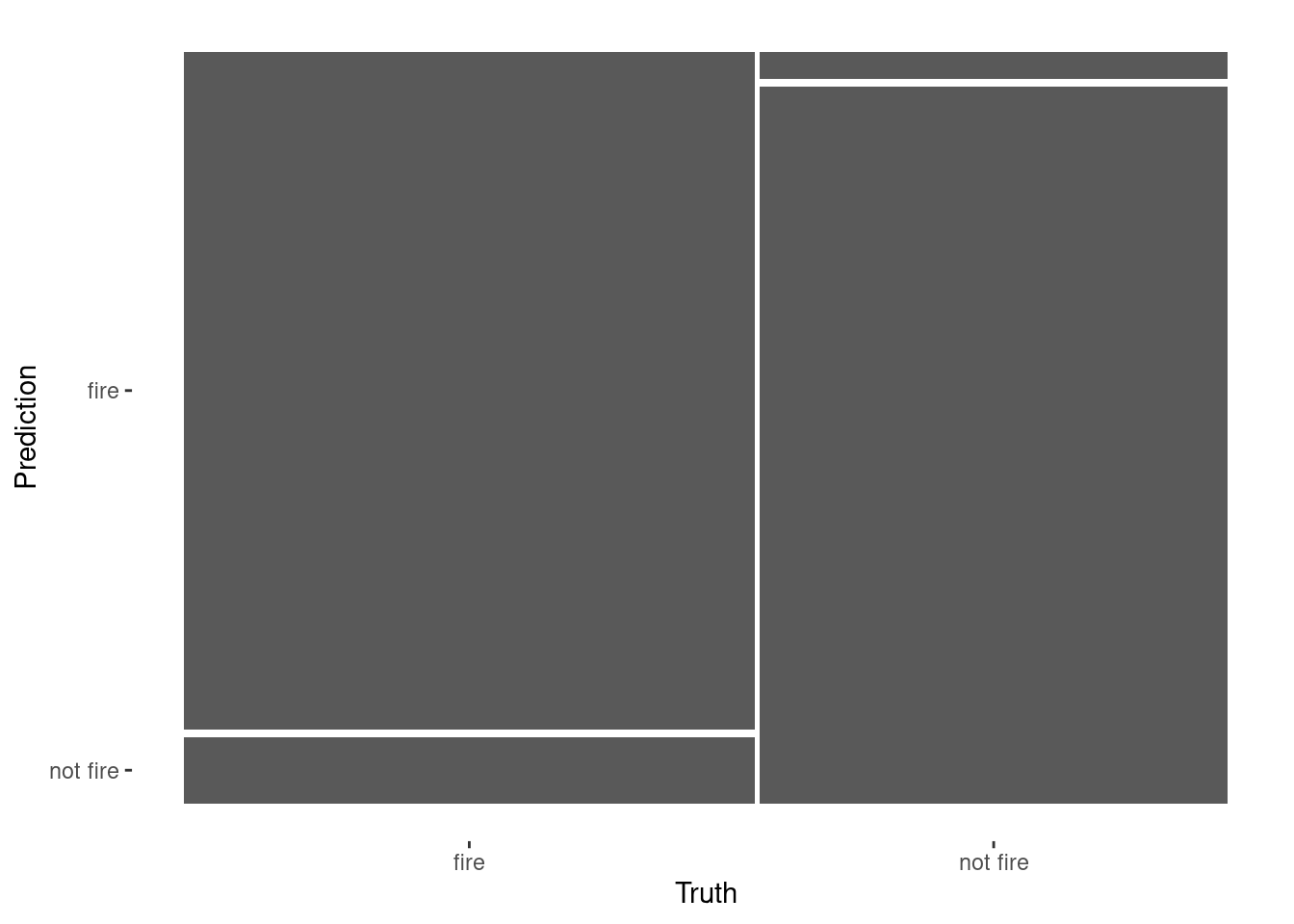
Confusion matrix: tabulation of true (i.e. expected) and predicted class labels

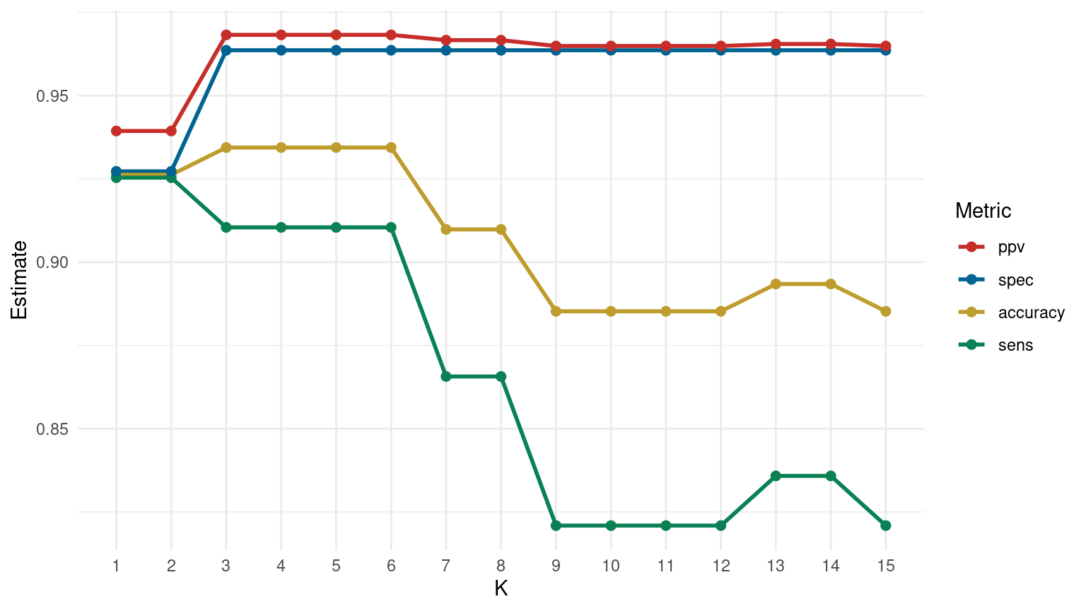
Performance metrics

Common metrics include:

• accuracy
• sensitivity
• specificity
• positive predictive value (PPV)

# code
conf_mat(fire_results, truth = classes, estimate = predicted) %>%  autoplot()

Accuracy

Proportion of correctly classified cases \[{\rm Accuracy} = \frac{\text{true positives} + \text{true negatives}}{n}\]

          Truth
Prediction fire not fire
  fire       61        2
  not fire    6       53

accuracy(fire_results, truth = classes, 
         estimate = predicted)

# A tibble: 1 × 3
  .metric  .estimator .estimate
  <chr>    <chr>          <dbl>
1 accuracy binary         0.934

Sensitivity

Proportion of positive cases that are predicted to be positive \[{\rm Sensitivity} = \frac{\text{true positives}}{ \text{true positives}+ \text{false negatives}}\] Also called… true positive rate or recall

          Truth
Prediction fire not fire
  fire       61        2
  not fire    6       53

sens(fire_results, truth = classes,
         estimate = predicted)

# A tibble: 1 × 3
  .metric .estimator .estimate
  <chr>   <chr>          <dbl>
1 sens    binary         0.910

Specificity

Proportion of negative cases that are predicted to be negative \[{\rm Specificity} = \frac{\text{true negatives}}{ \text{false positives}+ \text{true negatives}}\] Also called… true negative rate

          Truth
Prediction fire not fire
  fire       61        2
  not fire    6       53

spec(fire_results, truth = classes,
         estimate = predicted)

# A tibble: 1 × 3
  .metric .estimator .estimate
  <chr>   <chr>          <dbl>
1 spec    binary         0.964

Positive predictive value (PPV)

Proportion of cases that are predicted to be positives that are truly positives \[{\rm PPV} = \frac{\text{true positives}}{ \text{true positives} + \text{false positives}}\] Also called… precision

          Truth
Prediction fire not fire
  fire       61        2
  not fire    6       53

ppv(fire_results, truth = classes,
         estimate = predicted)

# A tibble: 1 × 3
  .metric .estimator .estimate
  <chr>   <chr>          <dbl>
1 ppv     binary         0.968

 Group Activity 2

• Please finish the remaining problems in the class activity for today

10:00

Tabulate the metrics !!

custom_metrics <- metric_set(accuracy, sens, spec, ppv) # select custom metrics
metrics <- custom_metrics(fire_results, truth = classes, estimate = predicted) 
metrics

# A tibble: 4 × 3
  .metric  .estimator .estimate
  <chr>    <chr>          <dbl>
1 accuracy binary         0.934
2 sens     binary         0.910
3 spec     binary         0.964
4 ppv      binary         0.968

Choose the optimal K based on majority of the metrics!

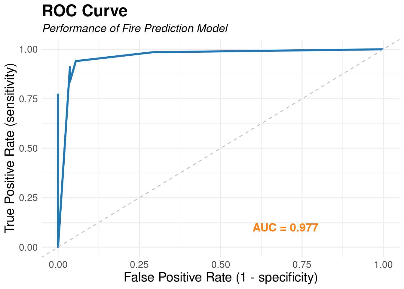
Receiver Operating Characteristic (ROC) curve

• ROC curve
• Code

library(yardstick)
fire_prob <- predict(fire_knn_fit, test_features, type = "prob")
fire_results2 <- fire_test %>% select(classes) %>% bind_cols(fire_prob)
fire_results2 %>%
  roc_curve(truth = classes, .pred_fire) %>%
  ggplot(aes(x = 1 - specificity, y = sensitivity)) +
  geom_line(color = "#1f77b4", size = 1.2) +
  geom_abline(linetype = "dashed", color = "gray") +
  annotate("text", x = 0.8, y = 0.1, label = paste("AUC =", round(roc_auc(fire_results2, truth = classes, .pred_fire)$.estimate, 3)), hjust = 1, color = "#ff7f0e", size = 5, fontface = "bold") +
  labs(title = "ROC Curve", subtitle = "Performance of Fire Prediction Model", x = "False Positive Rate (1 - specificity)", y = "True Positive Rate (sensitivity)") +
  theme_minimal()