Intro to Clustering

STAT 220

Bastola

Supervised learning


  • train or “supervise” algorithms to use labels to classify data or predict outcomes

  • use labeled inputs and outputs to measure model accuracy

Image source: click here

Unsupervised learning


  • uses statistical learning algorithms to analyze and cluster unlabeled data sets

  • discover hidden patterns in data without human intervention, so “unsupervised”

    • group unlabeled data based on their similarities or differences

Image source: click here

Example: get cluster association from unlabeled data

No labels!

Labels!!

Can use an unsupervised algorithm called k-means to achieve this!

K-means Basics


  • Algorithm to group data into K clusters

  • Starts with an initial clustering of data

  • Iteratively improves the cluster assignments

  • Stops until the assignments cannot be improved further

Algorithm


  1. Randomly assign a number, from 1 to K, to each of the observations

  2. Compute the centroid of each of the K clusters

  3. Assign each point to the nearest centroid and redefine the cluster

  4. Repeat steps 2 and 3 until no point change clusters

(1) Randomly assign a number, from 1 to K, to each of the observations

(2) Compute the centroid of each cluster

(3) Re-assign each observation to the cluster whose centroid is closest

(4) Re-compute the centroid of each cluster

(5) Re-assign each observation to the cluster whose centroid is closest

(6) Re-compute the centroid of each cluster

(7) Re-assign each observation to the cluster whose centroid is closest

(8) Re-compute the centroid of each cluster

(9) Re-assign each observation to the cluster whose centroid is closest

(10) Re-compute the centroid of each cluster

Main Idea

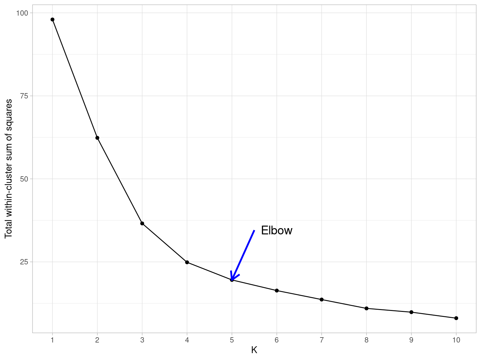
To minimize the total within cluster variation

The total within-cluster variation is the sum of squared Euclidean distances between items and the corresponding centroid:

\[WSS = \sum_{k=1}^K WSS(C_k) = \sum_{k=1}^K \sum_{x_i \in C_k}(x_i - \mu_k)^2\] where:

  • WSS is the Within Cluster Sum of Squared Errors
  • \(x_i\) is a data point in the cluster \(C_k\)
  • \(\mu_k\) is the mean value of the points assigned to the cluster \(C_k\)

USArrests

USAData <- as_tibble(USArrests, rownames = "state") %>% drop_na() %>%
  column_to_rownames("state") %>%
  select(Murder, UrbanPop)
USAData %>% knitr::kable()
Murder UrbanPop
Alabama 13.2 58
Alaska 10.0 48
Arizona 8.1 80
Arkansas 8.8 50
California 9.0 91
Colorado 7.9 78
Connecticut 3.3 77
Delaware 5.9 72
Florida 15.4 80
Georgia 17.4 60
Hawaii 5.3 83
Idaho 2.6 54
Illinois 10.4 83
Indiana 7.2 65
Iowa 2.2 57
Kansas 6.0 66
Kentucky 9.7 52
Louisiana 15.4 66
Maine 2.1 51
Maryland 11.3 67
Massachusetts 4.4 85
Michigan 12.1 74
Minnesota 2.7 66
Mississippi 16.1 44
Missouri 9.0 70
Montana 6.0 53
Nebraska 4.3 62
Nevada 12.2 81
New Hampshire 2.1 56
New Jersey 7.4 89
New Mexico 11.4 70
New York 11.1 86
North Carolina 13.0 45
North Dakota 0.8 44
Ohio 7.3 75
Oklahoma 6.6 68
Oregon 4.9 67
Pennsylvania 6.3 72
Rhode Island 3.4 87
South Carolina 14.4 48
South Dakota 3.8 45
Tennessee 13.2 59
Texas 12.7 80
Utah 3.2 80
Vermont 2.2 32
Virginia 8.5 63
Washington 4.0 73
West Virginia 5.7 39
Wisconsin 2.6 66
Wyoming 6.8 60

Means and standard deviations


USAData %>%
  map_dfr(~list(
    mean = mean(.x, na.rm = TRUE), 
    sd = sd(.x, na.rm = TRUE)
  ), .id = "variable")
# A tibble: 2 × 3
  variable  mean    sd
  <chr>    <dbl> <dbl>
1 Murder    7.79  4.36
2 UrbanPop 65.5  14.5 

Standardize the data

USAData <- USAData %>% mutate(across(where(is.numeric), standardize))
USAData %>% knitr::kable()
Murder UrbanPop
Alabama 1.2425641 -0.5209066
Alaska 0.5078625 -1.2117642
Arizona 0.0716334 0.9989801
Arkansas 0.2323494 -1.0735927
California 0.2782682 1.7589234
Colorado 0.0257146 0.8608085
Connecticut -1.0304190 0.7917228
Delaware -0.4334739 0.4462940
Florida 1.7476714 0.9989801
Georgia 2.2068599 -0.3827351
Hawaii -0.5712305 1.2062373
Idaho -1.1911350 -0.7972496
Illinois 0.5997002 1.2062373
Indiana -0.1350014 -0.0373063
Iowa -1.2829727 -0.5899924
Kansas -0.4105145 0.0317794
Kentucky 0.4389842 -0.9354212
Louisiana 1.7476714 0.0317794
Maine -1.3059321 -1.0045069
Maryland 0.8063350 0.1008652
Massachusetts -0.7778653 1.3444088
Michigan 0.9900104 0.5844655
Minnesota -1.1681755 0.0317794
Mississippi 1.9083874 -1.4881072
Missouri 0.2782682 0.3081225
Montana -0.4105145 -0.8663354
Nebraska -0.8008247 -0.2445636
Nevada 1.0129698 1.0680658
New Hampshire -1.3059321 -0.6590781
New Jersey -0.0890826 1.6207519
New Mexico 0.8292944 0.3081225
New York 0.7604162 1.4134946
North Carolina 1.1966452 -1.4190215
North Dakota -1.6044046 -1.4881072
Ohio -0.1120420 0.6535513
Oklahoma -0.2727580 0.1699510
Oregon -0.6630682 0.1008652
Pennsylvania -0.3416362 0.4462940
Rhode Island -1.0074596 1.4825804
South Carolina 1.5180772 -1.2117642
South Dakota -0.9156219 -1.4190215
Tennessee 1.2425641 -0.4518209
Texas 1.1277670 0.9989801
Utah -1.0533784 0.9989801
Vermont -1.2829727 -2.3171363
Virginia 0.1634711 -0.1754778
Washington -0.8697030 0.5153798
West Virginia -0.4793928 -1.8335360
Wisconsin -1.1911350 0.0317794
Wyoming -0.2268391 -0.3827351

kmeans() in R


  • kmeans() function takes a matrix or data-frame or tibble and the number of centers/clusters we want to find.

  • We also set nstart = 20-25 to have multiple initial starting positions in the hope of finding global optimal solution instead of local optimal solution

  • Use set.seed() for reproducibility

Within Cluster Sum of Squared Errors (WSS)

  • Calculate WSS for different values of K.

  • Choose K for which WSS first starts to diminish.

  • Visually deciphered with an elbow graph.

  • The number of clusters is taken at the elbow joint point.

K-means

set.seed(1234)
k.means <- kmeans(USAData, centers = 2, nstart = 25)
k.means
K-means clustering with 2 clusters of sizes 23, 27

Cluster means:
      Murder   UrbanPop
1  0.8961762  0.1939808
2 -0.7634094 -0.1652429

Clustering vector:
       Alabama         Alaska        Arizona       Arkansas     California 
             1              1              1              2              1 
      Colorado    Connecticut       Delaware        Florida        Georgia 
             1              2              2              1              1 
        Hawaii          Idaho       Illinois        Indiana           Iowa 
             2              2              1              2              2 
        Kansas       Kentucky      Louisiana          Maine       Maryland 
             2              1              1              2              1 
 Massachusetts       Michigan      Minnesota    Mississippi       Missouri 
             2              1              2              1              1 
       Montana       Nebraska         Nevada  New Hampshire     New Jersey 
             2              2              1              2              1 
    New Mexico       New York North Carolina   North Dakota           Ohio 
             1              1              1              2              2 
      Oklahoma         Oregon   Pennsylvania   Rhode Island South Carolina 
             2              2              2              2              1 
  South Dakota      Tennessee          Texas           Utah        Vermont 
             2              1              1              2              2 
      Virginia     Washington  West Virginia      Wisconsin        Wyoming 
             1              2              2              2              2 

Within cluster sum of squares by cluster:
[1] 31.59219 30.59764
 (between_SS / total_SS =  36.5 %)

Available components:

[1] "cluster"      "centers"      "totss"        "withinss"     "tot.withinss"
[6] "betweenss"    "size"         "iter"         "ifault"      

Tidy the information

k.means %>% broom::tidy()
# A tibble: 2 × 5
  Murder UrbanPop  size withinss cluster
   <dbl>    <dbl> <int>    <dbl> <fct>  
1  0.896    0.194    23     31.6 1      
2 -0.763   -0.165    27     30.6 2      
broom::glance(k.means)
# A tibble: 1 × 4
  totss tot.withinss betweenss  iter
  <dbl>        <dbl>     <dbl> <int>
1    98         62.2      35.8     1

augment the cluster identity

knitr::kable(broom::augment(k.means, data = USAData))
.rownames Murder UrbanPop .cluster
Alabama 1.2425641 -0.5209066 1
Alaska 0.5078625 -1.2117642 1
Arizona 0.0716334 0.9989801 1
Arkansas 0.2323494 -1.0735927 2
California 0.2782682 1.7589234 1
Colorado 0.0257146 0.8608085 1
Connecticut -1.0304190 0.7917228 2
Delaware -0.4334739 0.4462940 2
Florida 1.7476714 0.9989801 1
Georgia 2.2068599 -0.3827351 1
Hawaii -0.5712305 1.2062373 2
Idaho -1.1911350 -0.7972496 2
Illinois 0.5997002 1.2062373 1
Indiana -0.1350014 -0.0373063 2
Iowa -1.2829727 -0.5899924 2
Kansas -0.4105145 0.0317794 2
Kentucky 0.4389842 -0.9354212 1
Louisiana 1.7476714 0.0317794 1
Maine -1.3059321 -1.0045069 2
Maryland 0.8063350 0.1008652 1
Massachusetts -0.7778653 1.3444088 2
Michigan 0.9900104 0.5844655 1
Minnesota -1.1681755 0.0317794 2
Mississippi 1.9083874 -1.4881072 1
Missouri 0.2782682 0.3081225 1
Montana -0.4105145 -0.8663354 2
Nebraska -0.8008247 -0.2445636 2
Nevada 1.0129698 1.0680658 1
New Hampshire -1.3059321 -0.6590781 2
New Jersey -0.0890826 1.6207519 1
New Mexico 0.8292944 0.3081225 1
New York 0.7604162 1.4134946 1
North Carolina 1.1966452 -1.4190215 1
North Dakota -1.6044046 -1.4881072 2
Ohio -0.1120420 0.6535513 2
Oklahoma -0.2727580 0.1699510 2
Oregon -0.6630682 0.1008652 2
Pennsylvania -0.3416362 0.4462940 2
Rhode Island -1.0074596 1.4825804 2
South Carolina 1.5180772 -1.2117642 1
South Dakota -0.9156219 -1.4190215 2
Tennessee 1.2425641 -0.4518209 1
Texas 1.1277670 0.9989801 1
Utah -1.0533784 0.9989801 2
Vermont -1.2829727 -2.3171363 2
Virginia 0.1634711 -0.1754778 1
Washington -0.8697030 0.5153798 2
West Virginia -0.4793928 -1.8335360 2
Wisconsin -1.1911350 0.0317794 2
Wyoming -0.2268391 -0.3827351 2

In-built function for visuals using factoextra

library(factoextra)
fviz_cluster(k.means, data = USAData, repel = TRUE, 
             ggtheme = theme_tufte())

Determine the optimal number of clusters

set.seed(1234)
multi_kmeans <- tibble(k = 1:10) %>%
  mutate(
    model = purrr::map(k, ~ kmeans(USAData, centers = .x, nstart = 25)), 
    tot.withinss = purrr::map_dbl(model, ~ glance(.x)$tot.withinss) 
  )
multi_kmeans
# A tibble: 10 × 3
       k model    tot.withinss
   <int> <list>          <dbl>
 1     1 <kmeans>        98   
 2     2 <kmeans>        62.4 
 3     3 <kmeans>        36.6 
 4     4 <kmeans>        24.9 
 5     5 <kmeans>        19.6 
 6     6 <kmeans>        16.4 
 7     7 <kmeans>        13.7 
 8     8 <kmeans>        11.0 
 9     9 <kmeans>         9.85
10    10 <kmeans>         8.04

Determine the optimal number of clusters

set.seed(1234)
multi_kmeans <- tibble(k = 1:10) %>%
  mutate(
    model = purrr::map(k, ~ kmeans(USAData, centers = .x, nstart = 25)),
    tot.withinss = purrr::map_dbl(model, ~ glance(.x)$tot.withinss) 
  )

multi_kmeans
# A tibble: 10 × 3
       k model    tot.withinss
   <int> <list>          <dbl>
 1     1 <kmeans>        98   
 2     2 <kmeans>        62.4 
 3     3 <kmeans>        36.6 
 4     4 <kmeans>        24.9 
 5     5 <kmeans>        19.6 
 6     6 <kmeans>        16.4 
 7     7 <kmeans>        13.7 
 8     8 <kmeans>        11.0 
 9     9 <kmeans>         9.85
10    10 <kmeans>         8.04

Extract the centroids

USAData %>%
  mutate(Cluster = kmeans.final$cluster) %>%
  group_by(Cluster) %>%
  summarise_all("mean")
# A tibble: 5 × 3
  Cluster Murder UrbanPop
    <int>  <dbl>    <dbl>
1       1  1.17    -0.966
2       2 -1.09    -1.22 
3       3 -0.462    1.23 
4       4  1.07     0.746
5       5 -0.442    0.135

 Group Activity 1


  • Please clone the ca26-yourusername repository from Github
  • Please do problem 1 in the class activity for today

20:00