Data Objects in R

STAT 220

Bastola

Object Oriented Programming in R

R uses object-oriented programming (OOP) principles
Functions in R are designed to work with specific object classes and types
Example: plot() function behaves differently based on the input object

`plot()` Function Examples

Scatterplot with plot():

plot(y ~ x, data = mydata)  # If x and y are numeric, creates a scatterplot

Diagnostic plots with plot():

my_lm <- lm(y ~ x, data = mydata)  # Create a linear model
plot(my_lm)  # Produces diagnostic plots for the linear model

The plot() function adapts its behavior based on the input object’s class and type

Data structures and types in R

R objects are based on vectors
Two functions to examine objects:
- typeof(): Returns the storage mode (data type) of an object
- class(): Provides further description of an object
NULL: Represents an empty object (vector of length 0)

Examples of Data Types and Functions

Numeric and integer data types:

x <- c(8, 2, 1, 3)
typeof(x)  # "double" (numeric)

[1] "double"

x_int <- c(8L, 2L, 1L, 3L)
typeof(x_int)  # "integer"

[1] "integer"

Logical data type and class:

x_is_one <- x == 1
typeof(x_is_one)  # "logical"

[1] "logical"

object_class <- class(x_is_one)
object_class  # "numeric"

[1] "logical"

Atomic Vectors and lists

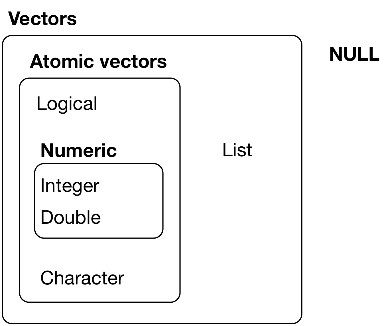
R uses two types of vectors to store info

atomic vectors: all entries have the same data type
lists: entries can contain other objects that can differ in data type

Examples of Vector Types

Atomic vector (numeric):

atomic_vector <- c(1, 2, 3, 4)
class(atomic_vector)  # "numeric"

[1] "numeric"

List with multiple data types:

my_list <- list(name = "John", age = 30, salary = 50000)
class(my_list)  # "list"

[1] "list"

Atomic Vectors: Matrices

You can add attributes, such as dimension, to vectors. A matrix is a 2-dimensional vector containing entries of the same type

Creating a matrix with dimensions:

my_matrix <- matrix(1:9, nrow = 3, ncol = 3)
class(my_matrix)  # "matrix"

[1] "matrix" "array"

my_matrix

     [,1] [,2] [,3]
[1,]    1    4    7
[2,]    2    5    8
[3,]    3    6    9

typeof(my_matrix)

[1] "integer"

Adding dimensions to a vector:

my_vector <- c(1, 2, 3, 4, 5, 6)
dim(my_vector) <- c(2, 3)
my_vector

     [,1] [,2] [,3]
[1,]    1    3    5
[2,]    2    4    6

class(my_vector)

[1] "matrix" "array"

typeof(my_vector)

[1] "double"

Creating Matrices Using Vector Binding

Bind vectors of the same length to create columns or rows. Use cbind() for column binding and rbind() for row binding

Column binding with cbind():

x <- c(1, 2, 3, 4)
x_col <- cbind(x = x, y = 2 * x)
x_col

     x y
[1,] 1 2
[2,] 2 4
[3,] 3 6
[4,] 4 8

Row binding with rbind():

x_row <- rbind(x1 = x, x2 = x * 2)
x_row

   [,1] [,2] [,3] [,4]
x1    1    2    3    4
x2    2    4    6    8

Implicit and Explicit Coercion in R

Implicit Coercion

R defaults to the most complex data type if more than one type is given

y <- c(1, 2, "a", NULL, TRUE)
typeof(y)

[1] "character"

class(y)

[1] "character"

[1] "1"    "2"    "a"    "TRUE"

Explicit coercion

Intentionally force a different data type from the “default” type

y <- as.character(c(1, 2, "a", NULL, TRUE))
typeof(y)

[1] "character"

class(y)

[1] "character"

[1] "1"    "2"    "a"    "TRUE"

Logical Vectors coercion

Logical values coerced into 0 for FALSE and 1 for TRUE when applying math functions

x <- c(8, 2, 1, 3)
x >= 5  # which entries >= 5?

[1]  TRUE FALSE FALSE FALSE

sum(x >= 5)  # how many >= 5?

[1] 1

Mean of a Logical Vector

mean(x >= 5)

[1] 0.25

Examples: Coercion of Logical Values

Sum of Logical Values

grades <- c(80, 60, 95, 70, 85)
passing_grades <- grades >= 65
sum(passing_grades)  # count of passing grades

[1] 4

Mean of Logical Values

rainfall <- c(2, 3, 5, 1, 9, 10)
rainy_days <- rainfall > 5
mean(rainy_days)  # proportion of rainy days

[1] 0.3333333

Data types: factors

Factors are a class of data that are stored as integers

x_fct <- as.factor(c("yes", 
                     "no", 
                     "no"))
class(x_fct)

[1] "factor"

typeof(x_fct)

[1] "integer"

levels(x_fct)

[1] "no"  "yes"

The attribute levels is a character vector of possible values

Values are stored as the integers (1=first level, 2=second level, etc.)
Levels are ordered alphabetically/numerically (unless specified otherwise)

Subsetting: Atomic Vector and Matrices

subset with [] by referencing index value (from 1 to vector length):

[1] 8 2 1 3

x[c(4, 2)]  # get 4th and 2nd entries

[1] 3 2

x[-c(4, 2)]  # omit 4th and 2nd entries

[1] 8 1

subset with a logical vector

# get 1st and 3rd entries
x[c(TRUE, FALSE, TRUE, FALSE)]

[1] 8 1

Subsetting: Matrices

Access entries using subsetting [row,column]

x_col

     x y
[1,] 1 2
[2,] 2 4
[3,] 3 6
[4,] 4 8

x_col[, 1] # first column

[1] 1 2 3 4

x_col[1:2, 1] # first 2 rows of first column

[1] 1 2

Subsetting: Atomic Vector and Matrices

x_df <- data.frame(x = x, 
                   double_x = x*2)
x_df

  x double_x
1 8       16
2 2        4
3 1        2
4 3        6

x_df[, 1]  # first column, all rows

[1] 8 2 1 3

or access columns with $

x_df$x  # get variable x column

[1] 8 2 1 3

# first column no longer a df
class(x_df[, 1])

[1] "numeric"

Tibbles

are a new modern data frame
never changes the input data types
can have columns that are lists
can have non-standard variable names
can start with a number or contain spaces

Subsetting data frames

Can also use column names to subset:

library(babynames)
# get 2 rows of Name and Sex
babynames[1:2, c("name", "sex")]

# A tibble: 2 × 2
  name  sex  
  <chr> <chr>
1 Mary  F    
2 Anna  F

Lists: Flexible Data Containers

List is a vector with entries that can be different object types

my_list <- list(myVec = x, 
                myDf = x_df, 
                myString = c("hi", "bye"))
my_list

$myVec
[1] 8 2 1 3

$myDf
  x double_x
1 8       16
2 2        4
3 1        2
4 3        6

$myString
[1] "hi"  "bye"

Accessing List Elements

Like a data frame, use the $ to access named objects stored in the list

my_list$myDf

  x double_x
1 8       16
2 2        4
3 1        2
4 3        6

class(my_list$myDf)

[1] "data.frame"

Subsetting Lists with Single Brackets

One [] operator gives you the object at the given location but preserves the list type
my_list[2] returns a list of length one with entry myDf

my_list[2]

$myDf
  x double_x
1 8       16
2 2        4
3 1        2
4 3        6

str(my_list[2])

List of 1
 $ myDf:'data.frame':   4 obs. of  2 variables:
  ..$ x       : num [1:4] 8 2 1 3
  ..$ double_x: num [1:4] 16 4 2 6

Subsetting Lists with Double Brackets

The double [[]] operator gives you the object stored at that location (equivalent to using $)
my_list[[2]] or my_list[["myDf"]] return the data frame myDf

my_list[[2]]

  x double_x
1 8       16
2 2        4
3 1        2
4 3        6

Please clone the ca3-yourusername repository from Github
Please do the problems on the class activity for today
Submit to Gradescope on moodle when done!

20:00

Data Objects in R

Object Oriented Programming in R

plot() Function Examples

Data structures and types in R

Examples of Data Types and Functions

Atomic Vectors and lists

Examples of Vector Types

Atomic Vectors: Matrices

Creating Matrices Using Vector Binding

Implicit and Explicit Coercion in R

Logical Vectors coercion

Examples: Coercion of Logical Values

Data types: factors

Subsetting: Atomic Vector and Matrices

Subsetting: Matrices

Subsetting: Atomic Vector and Matrices

Tibbles

Subsetting data frames

Lists: Flexible Data Containers

Accessing List Elements

Subsetting Lists with Single Brackets

Subsetting Lists with Double Brackets

Group Activity 1

`plot()` Function Examples