Tidy Data and Dates

STAT 220

Bastola

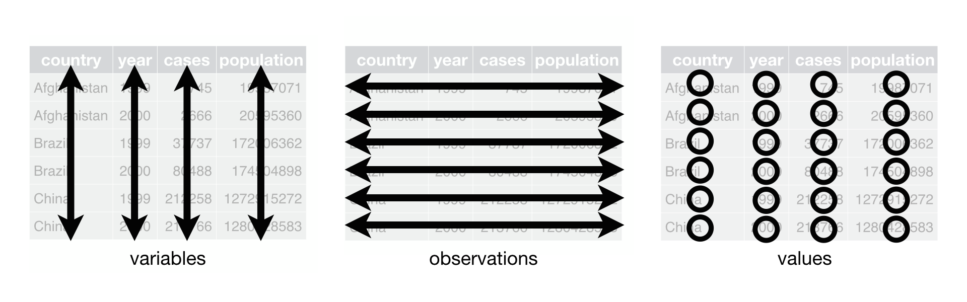
What are tidy data?

Each variable forms a column
Each observation forms a row
Each value has its own cell

Untidy data: example 1

untidy_data <- tibble(
  name = c("Ana","Bob","Cara"),
  wt_07_01_2021 = c(100, 150, 140),
  wt_08_01_2021 = c(104, 155, 138),
  wt_09_01_2021 = c(NA, 160, 142)
)

# A tibble: 3 × 4
  name  wt_07_01_2021 wt_08_01_2021 wt_09_01_2021
  <chr>         <dbl>         <dbl>         <dbl>
1 Ana             100           104            NA
2 Bob             150           155           160
3 Cara            140           138           142

Tidy data: example 1

library(tidyr)  # for tidying messy data
library(lubridate)  # for date manipulations
library(stringr) # for string manipulations
untidy_data %>% 
  pivot_longer(names_to = "date",  
               values_to = "weight", 
               cols = -name) %>%
  mutate(date = stringr::str_remove(date,"wt_"), 
         date = lubridate::dmy(date))

# A tibble: 9 × 3
  name  date       weight
  <chr> <date>      <dbl>
1 Ana   2021-01-07    100
2 Ana   2021-01-08    104
3 Ana   2021-01-09     NA
4 Bob   2021-01-07    150
5 Bob   2021-01-08    155
6 Bob   2021-01-09    160
7 Cara  2021-01-07    140
8 Cara  2021-01-08    138
9 Cara  2021-01-09    142

Wide data

Wide data has one row per subject, with multiple columns for their repeated measurements

Wide
id	SBP_visit1	SBP_visit2	SBP_visit3
a	132	100	111
b	120	106	112
c	130	126	128
d	118	116	108

Long data

Long data has multiple rows per subject, with one column for the measurement variable and another indicating from when/where the repeated measures are from

Long
id	visit	SBP
a	1	132
b	1	120
c	1	130
d	1	118
a	2	100
b	2	106
c	2	126
d	2	116
a	3	111
b	3	112
c	3	128
d	3	108

Wide to long: `pivot_longer()`

BP_wide

# A tibble: 4 × 5
  id    sex   SBP_v1 SBP_v2 SBP_v3
  <chr> <chr>  <dbl>  <dbl>  <dbl>
1 a     F        130    110    112
2 b     M        120    116    122
3 c     M        130    136    138
4 d     F        119    106    118

BP_long <- BP_wide %>%
  pivot_longer(names_to = "visit",  
               values_to = "SBP",  
               cols = SBP_v1:SBP_v3)   
BP_long

# A tibble: 12 × 4
   id    sex   visit    SBP
   <chr> <chr> <chr>  <dbl>
 1 a     F     SBP_v1   130
 2 a     F     SBP_v2   110
 3 a     F     SBP_v3   112
 4 b     M     SBP_v1   120
 5 b     M     SBP_v2   116
 6 b     M     SBP_v3   122
 7 c     M     SBP_v1   130
 8 c     M     SBP_v2   136
 9 c     M     SBP_v3   138
10 d     F     SBP_v1   119
11 d     F     SBP_v2   106
12 d     F     SBP_v3   118

Wide to long: `pivot_longer()`

pivot_longer lengthens data, increasing the number of rows and decreasing the number of columns.

Need to specify:

new column names
- names_to: stores row names of wide data’s columns
- .bvalues_to: stores data values
which columns to pivot

Long to wide: `pivot_wider()`

BP_long

# A tibble: 12 × 4
   id    sex   visit    SBP
   <chr> <chr> <chr>  <dbl>
 1 a     F     SBP_v1   130
 2 a     F     SBP_v2   110
 3 a     F     SBP_v3   112
 4 b     M     SBP_v1   120
 5 b     M     SBP_v2   116
 6 b     M     SBP_v3   122
 7 c     M     SBP_v1   130
 8 c     M     SBP_v2   136
 9 c     M     SBP_v3   138
10 d     F     SBP_v1   119
11 d     F     SBP_v2   106
12 d     F     SBP_v3   118

BP_wide1 <- BP_long %>% 
  pivot_wider(names_from = "visit", 
              values_from = "SBP") 
BP_wide1

# A tibble: 4 × 5
  id    sex   SBP_v1 SBP_v2 SBP_v3
  <chr> <chr>  <dbl>  <dbl>  <dbl>
1 a     F        130    110    112
2 b     M        120    116    122
3 c     M        130    136    138
4 d     F        119    106    118

Long to wide: `pivot_wider()`

pivot_wider increases number of columns and decreases the number of rows.

Need to specify:

new column names
- names_from: get the name of the column
- values_from: get the cell values from

Separate Info

BP_long

# A tibble: 12 × 4
   id    sex   visit    SBP
   <chr> <chr> <chr>  <dbl>
 1 a     F     SBP_v1   130
 2 a     F     SBP_v2   110
 3 a     F     SBP_v3   112
 4 b     M     SBP_v1   120
 5 b     M     SBP_v2   116
 6 b     M     SBP_v3   122
 7 c     M     SBP_v1   130
 8 c     M     SBP_v2   136
 9 c     M     SBP_v3   138
10 d     F     SBP_v1   119
11 d     F     SBP_v2   106
12 d     F     SBP_v3   118

BP_long1 <- BP_long %>%
  separate(visit, c("type", 
                    "visit")) 
BP_long1

# A tibble: 12 × 5
   id    sex   type  visit   SBP
   <chr> <chr> <chr> <chr> <dbl>
 1 a     F     SBP   v1      130
 2 a     F     SBP   v2      110
 3 a     F     SBP   v3      112
 4 b     M     SBP   v1      120
 5 b     M     SBP   v2      116
 6 b     M     SBP   v3      122
 7 c     M     SBP   v1      130
 8 c     M     SBP   v2      136
 9 c     M     SBP   v3      138
10 d     F     SBP   v1      119
11 d     F     SBP   v2      106
12 d     F     SBP   v3      118

`readr::parse_number()`

Goal: Extract first number from the visit column and remove the characters

BP_long

# A tibble: 12 × 4
   id    sex   visit    SBP
   <chr> <chr> <chr>  <dbl>
 1 a     F     SBP_v1   130
 2 a     F     SBP_v2   110
 3 a     F     SBP_v3   112
 4 b     M     SBP_v1   120
 5 b     M     SBP_v2   116
 6 b     M     SBP_v3   122
 7 c     M     SBP_v1   130
 8 c     M     SBP_v2   136
 9 c     M     SBP_v3   138
10 d     F     SBP_v1   119
11 d     F     SBP_v2   106
12 d     F     SBP_v3   118

BP_long2 <- BP_long %>% 
  mutate(visit = parse_number(visit)) 
BP_long2

# A tibble: 12 × 4
   id    sex   visit   SBP
   <chr> <chr> <dbl> <dbl>
 1 a     F         1   130
 2 a     F         2   110
 3 a     F         3   112
 4 b     M         1   120
 5 b     M         2   116
 6 b     M         3   122
 7 c     M         1   130
 8 c     M         2   136
 9 c     M         3   138
10 d     F         1   119
11 d     F         2   106
12 d     F         3   118

Make cleaned-up long data wide

head(BP_long2, 4)

# A tibble: 4 × 4
  id    sex   visit   SBP
  <chr> <chr> <dbl> <dbl>
1 a     F         1   130
2 a     F         2   110
3 a     F         3   112
4 b     M         1   120

BP_wide2 <- BP_long2 %>% 
  pivot_wider(names_from = "visit", 
              values_from = "SBP") 
BP_wide2

# A tibble: 4 × 5
  id    sex     `1`   `2`   `3`
  <chr> <chr> <dbl> <dbl> <dbl>
1 a     F       130   110   112
2 b     M       120   116   122
3 c     M       130   136   138
4 d     F       119   106   118

Problem: have numbers as column names
Solution: have row names start with the key column’s name separated by a character

BP_wide3 <- BP_long2 %>% 
  pivot_wider(names_from = "visit",     
              values_from = "SBP",      
              names_prefix = "value_")  
BP_wide3

# A tibble: 4 × 5
  id    sex   value_1 value_2 value_3
  <chr> <chr>   <dbl>   <dbl>   <dbl>
1 a     F         130     110     112
2 b     M         120     116     122
3 c     M         130     136     138
4 d     F         119     106     118

Please clone the ca8-yourusername repository from Github
Please do the problem 1 in the class activity for today

10:00

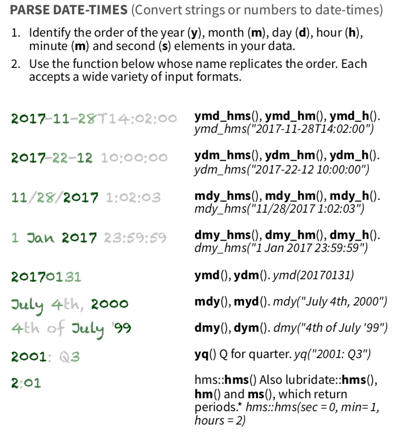
Dates with `lubridate`

Convert characters to special “Date” type
Easy date magic examples:
- add and subtract dates
- convert to minutes/years/etc
- change timezones
- add 1 month to a date…

Allison Horst

What kind of date do you have?

Parsing Complex Dates

library(lubridate)
complex_dates <- tibble(
  name = c("Yi", "Mo", "Dee"),
  dob = c("31-October-1952 14:30:15",
          "12-Jan-1984 22:15:00",
          "02-Feb-2002 10:45:30")
)

complex_dates %>%
  mutate(dob_date = dmy_hms(dob)) %>% 
  knitr::kable()  # to make nice tables

name	dob	dob_date
Yi	31-October-1952 14:30:15	1952-10-31 14:30:15
Mo	12-Jan-1984 22:15:00	1984-01-12 22:15:00
Dee	02-Feb-2002 10:45:30	2002-02-02 10:45:30

Advanced Date Arithmetic

complex_dates %>%
  mutate( dob_date = dmy_hms(dob),
          dob_year = year(dob_date),
          time_since_birth = interval(dob_date, now()),
          age_exact = time_length(time_since_birth, unit = "years")) %>%
  knitr::kable()

name	dob	dob_date	dob_year	time_since_birth	age_exact
Yi	31-October-1952 14:30:15	1952-10-31 14:30:15	1952	1952-10-31 14:30:15 UTC–2024-05-15 03:37:38 UTC	71.53701
Mo	12-Jan-1984 22:15:00	1984-01-12 22:15:00	1984	1984-01-12 22:15:00 UTC–2024-05-15 03:37:38 UTC	40.33668
Dee	02-Feb-2002 10:45:30	2002-02-02 10:45:30	2002	2002-02-02 10:45:30 UTC–2024-05-15 03:37:38 UTC	22.28061

Advanced Date Arithmetic: alternate

complex_dates %>%
  mutate(dob_date = dmy_hms(dob),
        age_exact = as.numeric(interval(dob_date, now()) / years(1))) %>% 
  knitr::kable()

name	dob	dob_date	age_exact
Yi	31-October-1952 14:30:15	1952-10-31 14:30:15	71.53701
Mo	12-Jan-1984 22:15:00	1984-01-12 22:15:00	40.33668
Dee	02-Feb-2002 10:45:30	2002-02-02 10:45:30	22.28061

Creating Date-Time Objects with `make_datetime()`

# Components of date and time
year_component <- 2024
month_component <- 1
day_component <- 19
hour_component <- 9
minute_component <- 03
second_component <- 30

# Create a date-time object
date_time_object <- make_datetime(
  year = year_component,
  month = month_component,
  day = day_component,
  hour = hour_component,
  min = minute_component,
  sec = second_component
)

date_time_object

[1] "2024-01-19 09:03:30 UTC"

Advanced Date-Time Arithmetic

date_time <- tibble(date = ymd("2024-01-13", "2024-03-06", "2025-06-30"))

date_time %>%
  mutate(add_month = date %m+% months(1), 
         add_year = date %m+% years(1),
         subtract_week = date %m-% weeks(1)) %>% 
  knitr::kable()

date	add_month	add_year	subtract_week
2024-01-13	2024-02-13	2025-01-13	2024-01-06
2024-03-06	2024-04-06	2025-03-06	2024-02-28
2025-06-30	2025-07-30	2026-06-30	2025-06-23

Duration and Time Differences

time_diff_example <- tibble(
  start_date = ymd("2024-01-03"),
  end_date = ymd("2024-03-17")
)

time_diff_example %>%
  mutate(time_diff = end_date - start_date,
         duration_days = time_length(time_diff, unit = "days"),
         duration_weeks = as.duration(time_diff) / dweeks(1),
         duration_months = as.duration(time_diff) / dmonths(1),
         duration_years = as.duration(time_diff) / dyears(1))  %>% 
  knitr::kable()

start_date	end_date	time_diff	duration_days	duration_weeks	duration_months	duration_years
2024-01-03	2024-03-17	74 days	74	10.57143	2.431211	0.202601

Please do the remaining problems in the class activity.
Submit to Gradescope on moodle when done!

10:00

id	visit	SBP
a	1	132
b	1	120
c	1	130
d	1	118
a	2	100
b	2	106
c	2	126
d	2	116
a	3	111
b	3	112
c	3	128
d	3	108

id	visit	SBP
a	1	132
b	1	120
c	1	130
d	1	118
a	2	100
b	2	106
c	2	126
d	2	116
a	3	111
b	3	112
c	3	128
d	3	108

Tidy Data and Dates

What are tidy data?

Untidy data: example 1

Tidy data: example 1

Wide data

Long data

Wide to long: pivot_longer()

Wide to long: pivot_longer()

Long to wide: pivot_wider()

Long to wide: pivot_wider()

Separate Info

readr::parse_number()

Make cleaned-up long data wide

Group Activity 1

Dates with lubridate

What kind of date do you have?

Parsing Complex Dates

Advanced Date Arithmetic

Advanced Date Arithmetic: alternate

Creating Date-Time Objects with make_datetime()

Advanced Date-Time Arithmetic

Duration and Time Differences

Group Activity 2

Wide to long: `pivot_longer()`

Wide to long: `pivot_longer()`

Long to wide: `pivot_wider()`

Long to wide: `pivot_wider()`

`readr::parse_number()`

Dates with `lubridate`

Creating Date-Time Objects with `make_datetime()`

id	visit	SBP
a	1	132
b	1	120
c	1	130
d	1	118
a	2	100
b	2	106
c	2	126
d	2	116
a	3	111
b	3	112
c	3	128
d	3	108