#install.packages("babynames")  # uncomment to install
library(babynames)Class Activity 1
The R package babynames provides data about the popularity of individual baby names from the US Social Security Administration. Data includes all names used at least 5 times in a year beginning in 1880.
Below is the list for first few cases of baby names.
head(babynames)# A tibble: 6 × 5
year sex name n prop
<dbl> <chr> <chr> <int> <dbl>
1 1880 F Mary 7065 0.0724
2 1880 F Anna 2604 0.0267
3 1880 F Emma 2003 0.0205
4 1880 F Elizabeth 1939 0.0199
5 1880 F Minnie 1746 0.0179
6 1880 F Margaret 1578 0.0162- How many cases and variables are in the dataset
babynames?
Answer:
To determine the number of cases (rows) and variables (columns) in the dataset, we can use the dim() function, which returns the dimensions of the dataset.
dim(babynames)[1] 1924665 5There are 2,020,863 cases (rows) and 5 variables (columns) in the dataset babynames.
Let’s use the package tidyverse to do some exploratory data analysis.
#install.packages("tidyverse")   # uncomment to install
library(tidyverse)
babynames %>% filter(name=='Aimee')
# A tibble: 150 × 5
year sex name n prop
<dbl> <chr> <chr> <int> <dbl>
1 1880 F Aimee 13 0.000133
2 1881 F Aimee 11 0.000111
3 1882 F Aimee 13 0.000112
4 1883 F Aimee 11 0.0000916
5 1884 F Aimee 15 0.000109
6 1885 F Aimee 17 0.000120
7 1886 F Aimee 17 0.000111
8 1887 F Aimee 18 0.000116
9 1888 F Aimee 12 0.0000633
10 1889 F Aimee 16 0.0000846
# ℹ 140 more rowsfiltered_names <- babynames %>% filter(name=='Aimee')#install.packages("ggplot2") # uncomment to install
library(ggplot2)ggplot(data=filtered_names, aes(x=year, y=prop)) +
geom_line(aes(colour=sex)) +
xlab('Year') +
ylab('Prop. of Babies Named Aimee')
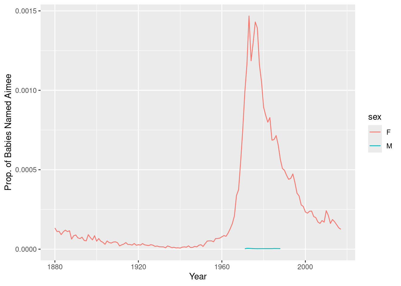
- What do you see in the Figure 1? Explain in a few sentences.
Answer:
Figure 1 shows the trend of the proportion of babies named Aimee over the years, separated by sex. We can observe that the name Aimee was more popular for girls compared to boys throughout the years. The name’s popularity increased from the early 1900s, reaching its peak around the 1970s, and then declined. The proportion of boys named Aimee remained consistently low across the years.
- Repeat question 2 to infer how does the proportion of babies with your first name trends over time.
Answer:
Replace “YourName” with your actual first name in the code below:
# Your R-code
your_name <- "Yourname"
your_name_data <- babynames %>% filter(name == your_name)

ggplot(data=your_name_data, aes(x=year, y=prop)) +
  geom_line(aes(colour=sex)) +
  xlab('Year') +
  ylab(paste0('Prop. of Babies Named ', your_name))
Examine the generated plot and describe the trend of your name’s popularity over time. Consider the following points:
Has the popularity of your name increased, decreased, or remained stable over the years? Is there a noticeable difference in popularity between sexes? Are there any interesting patterns or trends, such as sudden increases or decreases in popularity?
set.seed(123) # Set a seed for reproducibility
random_name <- sample(unique(babynames$name), 1)
random_name
[1] "Averyl"Now, replace ‘YourName’ with your first name and ‘RandomName’ with the randomly chosen name from the previous code:
your_name_data <- babynames %>% filter(name == 'Dee')
random_name_data <- babynames %>% filter(name == random_name)

combined_data <- bind_rows(your_name_data, random_name_data)

ggplot(data=combined_data, aes(x=year, y=prop)) +
  geom_line(aes(colour=sex, linetype=name)) +
  xlab('Year') +
  ylab('Proportion of Babies Named') +
  theme_minimal() +
  facet_wrap(~name, scales = "free_y")
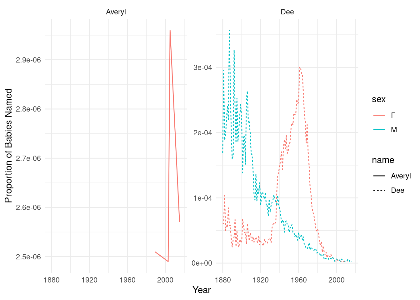
Examine the generated plot and compare the popularity of your first name with the randomly chosen name. Consider the following points:
Are there differences in popularity trends between the two names? Is one name consistently more popular than the other, or do their popularity levels change over time? Are there any interesting patterns or trends in the data, such as periods of rapid increase or decrease in popularity?