Class Activity 21

# load the necessary libraries
library(tidyverse) 
library(tidymodels)
library(mlbench)     
library(janitor)
library(paletteer)
library(corrr)
library(forcats)
library(ggthemes)

Group Activity 1

# Load the data
data(PimaIndiansDiabetes2)
db <- PimaIndiansDiabetes2 %>% drop_na()

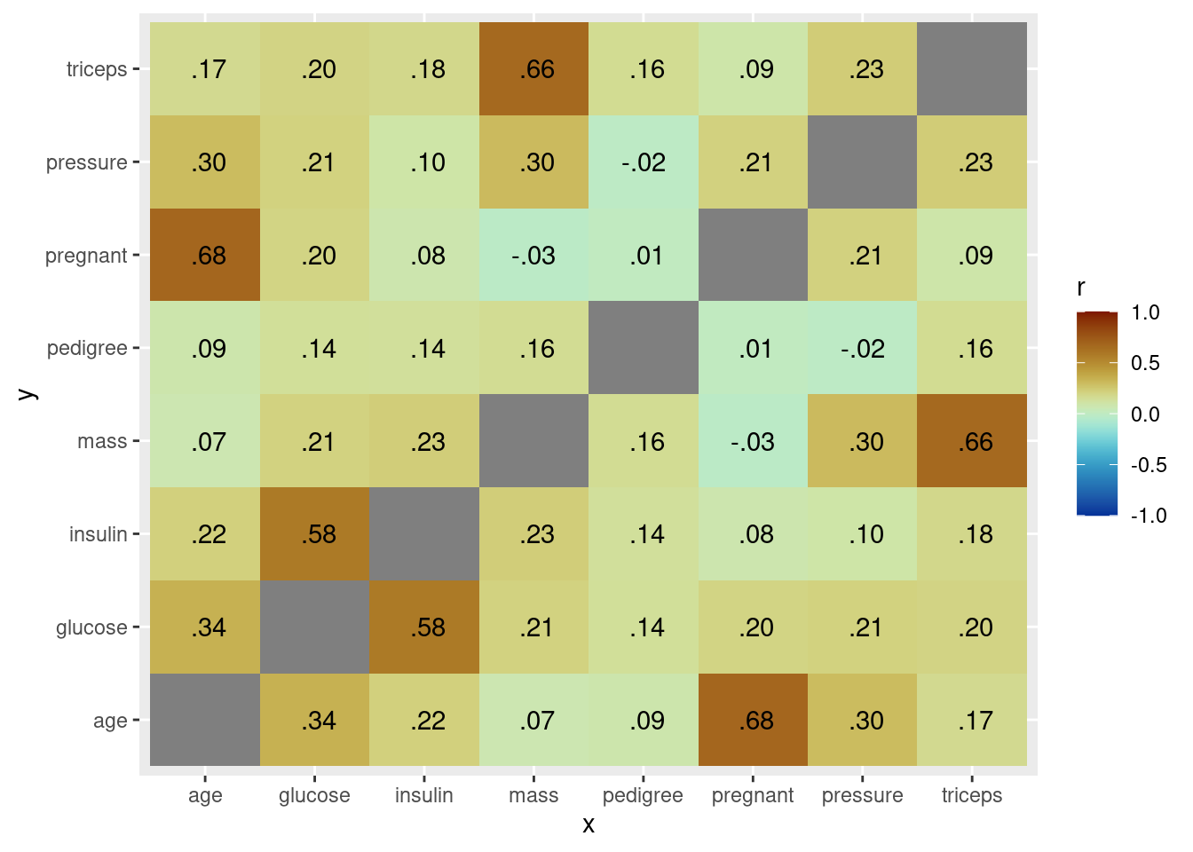
# correlation plot of the variables
db %>%
  select(-diabetes) %>%  # only numerical variables
  correlate() %>%
  stretch() %>%
  ggplot(aes(x, y, fill = r)) +
  geom_tile() +
  geom_text(aes(label = as.character(fashion(r)))) +
  scale_fill_paletteer_c("scico::roma", limits = c(-1, 1), direction = -1)

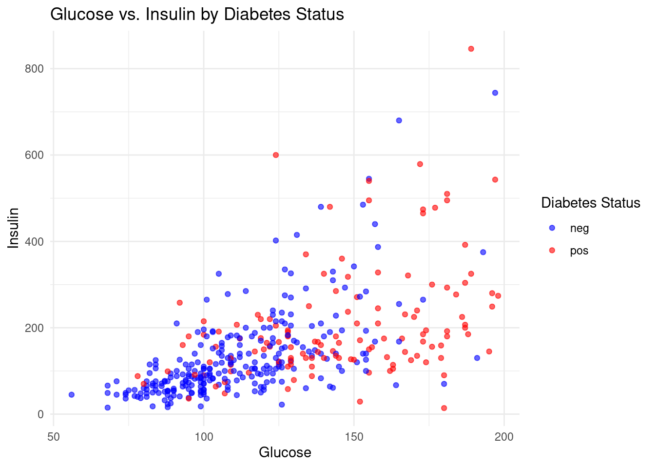
Create a scatter plot using ggplot2 to visualize the classification of diabetes status based on glucose and insulin levels, color-coding negative cases in blue and positive cases in red.

ggplot(db, aes(x = glucose, y = insulin, color = diabetes)) +
  geom_point(alpha = 0.6) +
  theme_minimal() + 
  labs(title = "Glucose vs. Insulin by Diabetes Status",
       x = "Glucose",
       y = "Insulin",
       color = "Diabetes Status") + 
  scale_color_manual(values = c("neg" = "blue", "pos" = "red"))

Using the provided standardization function, apply it to both the glucose and insulin columns of your dataset to create new standardized columns, then plot these standardized values to analyze diabetes status.

# function that standardizes
standardize <- function(x, na.rm = FALSE) {
  (x - mean(x, na.rm = na.rm)) / 
    sd(x, na.rm = na.rm)
}

db_std <- db %>%
  mutate(glucose_std = standardize(glucose),
         insulin_std = standardize(insulin))

Let’s perform all the steps involved in classifying whether a patient with certain glucose and insulin would have diabetes or not.

Click for answer

Answer:

# 1 Prepare raw data
db_raw <- db  %>%  select(glucose, insulin, diabetes)

# 2 Create a recipe for data pre-processing
db_recipe <- recipe(diabetes ~ glucose + insulin, data = db_raw) %>%
  step_scale(all_predictors()) %>%
  step_center(all_predictors()) %>%
  prep()

# 3 Apply the recipe to the data set
db_scaled <-  bake(db_recipe, db_raw)

# 4 Create a model specification
knn_spec <- nearest_neighbor(mode = "classification",
                             engine = "kknn",
                             neighbors = 5)

# 5 Fit the model on the pre-processed data
knn_fit <- knn_spec %>%
 fit(diabetes ~ insulin + diabetes, data = db_scaled)

# 6 Classify
# These are standardized value!!
new_observations <- tibble(glucose = c(1, 2), insulin = c(-1, 1))
predict(knn_fit, new_data = new_observations)

# A tibble: 2 × 1
  .pred_class
  <fct>      
1 neg        
2 neg

We already know the labels of the patients in the dataset. How well does the model predict their diabetes status?

Click for answer

Answer:

scaled_observations <- db_scaled[1:50,]
predictions <- predict(knn_fit, new_data = scaled_observations)
bind_cols(scaled_observations, predictions) -> predict_data

What is the accuracy percentage?

Answer:

sum(predictions == db_raw %>% select(diabetes) %>% slice(1:50))/50

[1] 0.9

# alternate
accuracy_percentage <- predict_data %>%
  mutate(correct_prediction = diabetes == .pred_class) %>%
  summarize(accuracy = mean(correct_prediction, na.rm = TRUE)) %>%
  pull(accuracy) * 100

accuracy_percentage

[1] 90

Repeat part d. with a different model fitted with different number of neighbors. See if the accuracy percentage change in this new setting.

Click for answer

Answer:

knn_spec <- nearest_neighbor(mode = "classification",
                             engine = "kknn",
                             weight_func = "rectangular",
                             neighbors = 2)
knn_fit <- knn_spec %>%
 fit(diabetes ~ ., data = db_scaled)

scaled_observations <- db_scaled
predictions <- predict(knn_fit, new_data = scaled_observations)

bind_cols(scaled_observations, predictions) -> predict_data

# accuracy percentage
accuracy_percentage <- predict_data %>%
  mutate(correct_prediction = diabetes == .pred_class) %>%
  summarize(accuracy = mean(correct_prediction, na.rm = TRUE)) %>%
  pull(accuracy) * 100

accuracy_percentage

[1] 100