# load the necessary libraries
library(tidyverse)
library(stringr)
library(polite)
library(rvest)Class Activity 16
Group Activity 1
a. Scrape the first table in List_of_NASA_missions wiki page. Additionally, use janitor::clean_names() to clean the column names and store the resulting table as NASA_missions.csv in your working folder.
Click for answer
wiki_NASA <- "https://en.wikipedia.org/wiki/List_of_NASA_missions"

# Scrape the data and write the first table to a CSV file
bow(wiki_NASA) %>%
  scrape() %>%
  html_nodes("table") %>%
  .[[1]] %>%
  html_table(fill = TRUE) %>%
  janitor::clean_names() %>%
write_csv("NASA_missions.csv")Group Activity 2
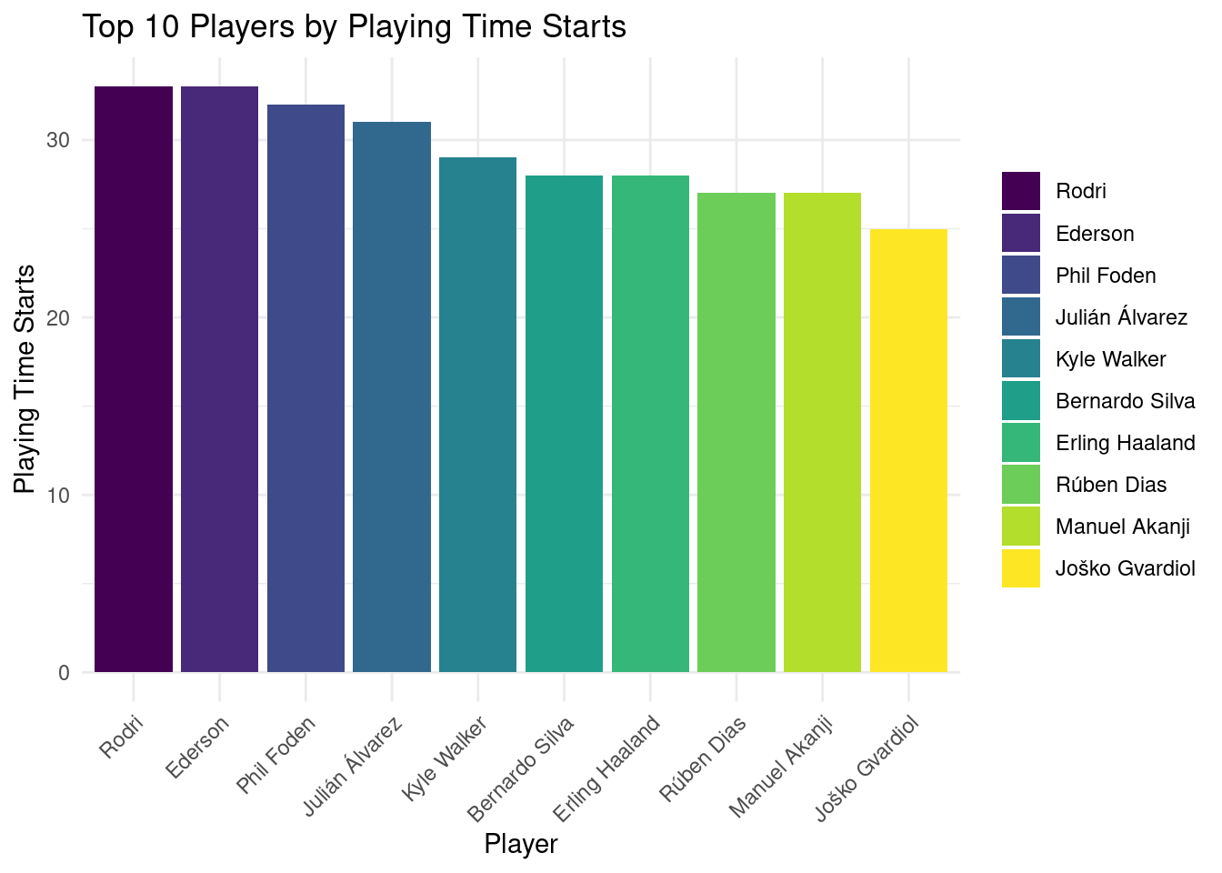
a. Scrape player statistics from the given web page, clean and reformat the data table headers using R packages, and create a bar chart to display the top ten players by playing time starts.
Start by extracting a table from a webpage using the rvest package, then clean the headers by merging them with subheaders and using janitor to standardize the names.
Click for answer
mancity <- "https://fbref.com/en/squads/b8fd03ef/Manchester-City-Stats"

data <- bow(mancity) %>%
  scrape() %>%
  html_nodes(css = "table") %>%
  html_table() %>%
  .[[1]]
data
# A tibble: 33 × 34
`` `` `` `` `` `Playing Time` `Playing Time` `Playing Time`
<chr> <chr> <chr> <chr> <chr> <chr> <chr> <chr>
1 Player Nati… Pos Age MP Starts Min 90s
2 Rodri es E… MF 27-3… 33 33 2,841 31.6
3 Ederson br B… GK 30-2… 33 33 2,785 30.9
4 Phil Fo… eng … FW,MF 23-3… 34 32 2,768 30.8
5 Julián … ar A… MF,FW 24-1… 36 31 2,647 29.4
6 Kyle Wa… eng … DF 33-3… 31 29 2,677 29.7
7 Bernard… pt P… MF,FW 29-2… 32 28 2,488 27.6
8 Erling … no N… FW 23-2… 30 28 2,462 27.4
9 Rúben D… pt P… DF 27-0… 29 27 2,469 27.4
10 Manuel … ch S… DF,MF 28-3… 29 27 2,441 27.1
# ℹ 23 more rows
# ℹ 26 more variables: Performance <chr>, Performance <chr>, Performance <chr>,
# Performance <chr>, Performance <chr>, Performance <chr>, Performance <chr>,
# Performance <chr>, Expected <chr>, Expected <chr>, Expected <chr>,
# Expected <chr>, Progression <chr>, Progression <chr>, Progression <chr>,
# `Per 90 Minutes` <chr>, `Per 90 Minutes` <chr>, `Per 90 Minutes` <chr>,
# `Per 90 Minutes` <chr>, `Per 90 Minutes` <chr>, `Per 90 Minutes` <chr>, …data_clean <- data %>%
{ subheaders <- .[1, ]
new_names <- map2_chr(names(.), subheaders, ~ str_c(.x, .y, sep = "-"))
setNames(., new_names)
}
data_clean %>% janitor::clean_names() %>%
slice(-1, -n(), -n()+1) -> data_clean
data_clean # A tibble: 30 × 34
player nation pos age mp playing_time_starts playing_time_min
<chr> <chr> <chr> <chr> <chr> <chr> <chr>
1 Rodri es ESP MF 27-3… 33 33 2,841
2 Ederson br BRA GK 30-2… 33 33 2,785
3 Phil Foden eng ENG FW,MF 23-3… 34 32 2,768
4 Julián Álvarez ar ARG MF,FW 24-1… 36 31 2,647
5 Kyle Walker eng ENG DF 33-3… 31 29 2,677
6 Bernardo Silva pt POR MF,FW 29-2… 32 28 2,488
7 Erling Haaland no NOR FW 23-2… 30 28 2,462
8 Rúben Dias pt POR DF 27-0… 29 27 2,469
9 Manuel Akanji ch SUI DF,MF 28-3… 29 27 2,441
10 Joško Gvardiol hr CRO DF 22-1… 27 25 2,238
# ℹ 20 more rows
# ℹ 27 more variables: playing_time_90s <chr>, performance_gls <chr>,
# performance_ast <chr>, performance_g_a <chr>, performance_g_pk <chr>,
# performance_pk <chr>, performance_p_katt <chr>, performance_crd_y <chr>,
# performance_crd_r <chr>, expected_x_g <chr>, expected_npx_g <chr>,
# expected_x_ag <chr>, expected_npx_g_x_ag <chr>, progression_prg_c <chr>,
# progression_prg_p <chr>, progression_prg_r <chr>, …Analyze the ‘playing_time_starts’ to find the top ten players and visualize this data in a bar chart using ggplot2, ensuring the chart is both informative and aesthetically pleasing.
data_clean_plot <- data_clean %>%
  mutate(
    playing_time_starts = readr::parse_number(playing_time_starts),
    player = factor(player, levels = player)
  ) %>%
  arrange(desc(playing_time_starts)) %>%
  top_n(10, playing_time_starts)

ggplot(data_clean_plot, aes(x = reorder(player, -playing_time_starts), y = playing_time_starts, fill = player)) +
  geom_bar(stat = "identity") +
  labs(title = "Top 10 Players by Playing Time Starts",
       x = "Player",
       y = "Playing Time Starts") +
  theme_minimal() +
  theme(axis.text.x = element_text(angle = 45, hjust = 1),
        legend.title = element_blank()) +
scale_fill_viridis_d() 
Group Activity 3
In this activity, you’ll scrape web data using rvest and tidy up the results into a well-formatted table. Start by extracting job titles from a given URL, then gather the associated company names, and trim any leading or trailing whitespace from the location data. Next, retrieve the posting dates and the URLs for the full job descriptions. Finally, combine all these elements into a single dataframe, ensuring that each piece of information aligns correctly. Your task is to produce a clean and informative table that could be useful for job seekers. To facilitate the selection of the correct CSS selectors, you may find the SelectorGadget Chrome extension particularly useful.
url <- "https://realpython.github.io/fake-jobs/"Click for answer
title <- bow(url) %>% scrape() %>% html_elements(css = ".is-5") %>% html_text()   # part 1
company <- bow(url) %>% scrape() %>% html_elements(css = ".company") %>% html_text() # part 2
location <- bow(url) %>% scrape() %>% html_elements(css = ".location") %>% html_text() %>% str_trim() # part 3
time <- bow(url) %>% scrape() %>% html_elements(css = "time") %>% html_text() # part 4
html <- bow(url) %>% scrape() %>%  html_element(css = ".card-footer-item+ .card-footer-item") %>% html_attr("href")  # part 5

# Create a dataframe
tibble(title = title, company = company, location = location, time = time, html = html) # port 6
# A tibble: 100 × 5
title company location time html
<chr> <chr> <chr> <chr> <chr>
1 Senior Python Developer Payne, Roberts and Davis Stewartbury… 2021… http…
2 Energy engineer Vasquez-Davidson Christopher… 2021… http…
3 Legal executive Jackson, Chambers and Levy Port Ericab… 2021… http…
4 Fitness centre manager Savage-Bradley East Seanvi… 2021… http…
5 Product manager Ramirez Inc North Jamie… 2021… http…
6 Medical technical officer Rogers-Yates Davidville,… 2021… http…
7 Physiological scientist Kramer-Klein South Chris… 2021… http…
8 Textile designer Meyers-Johnson Port Jonath… 2021… http…
9 Television floor manager Hughes-Williams Osbornetown… 2021… http…
10 Waste management officer Jones, Williams and Villa Scotttown, … 2021… http…
# ℹ 90 more rows