# load the necessary libraries
library(tidyverse)
library(tidymodels)
library(mlbench)     # for PimaIndiansDiabetes2 dataset
library(janitor)
library(parsnip)
library(kknn)
library(ggthemes)
library(purrr)
library(forcats)Class Activity 22
Group Activity 1
Load the mlbench package to get PimaIndiansDiabetes2 dataset.
# Load the data - diabetes
data(PimaIndiansDiabetes2)
db <- PimaIndiansDiabetes2
db <- db %>% drop_na() %>% mutate(diabetes = fct_rev(factor(diabetes)))
db_raw <- db %>% select(glucose, insulin, diabetes)- Split the data
75-25into training and test set using the following code.
Click for answer
Answer:
set.seed(123)

db_split <- initial_split(db, prop = 0.75)

# Create training data
db_train <- db_split %>% training()

# Create testing data
db_test <- db_split %>% testing()- Follow the steps to train a 7-NN classifier using the
tidymodelstoolkit
Click for answer
Answer:
# define recipe and preprocess the data
db_recipe <- recipe(diabetes ~ ., data = db_raw) %>%
  step_scale(all_predictors()) %>%
  step_center(all_predictors())
# specify the model
db_knn_spec7 <- nearest_neighbor(mode = "classification",
engine = "kknn",
weight_func = "rectangular",
neighbors = 7)# define the workflow
db_workflow <- workflow() %>%
add_recipe(db_recipe) %>%
add_model(db_knn_spec7)# fit the model
db_fit <- fit(db_workflow, data = db_train)- Classify the penguins in the
testdata frame.
Click for answer
Answer:
test_features <- db_test %>% select(glucose, insulin)
db_pred <- predict(db_fit, test_features, type = "raw")

db_results <- db_test %>%
  select(glucose, insulin, diabetes) %>%
  bind_cols(predicted = db_pred)

head(db_results, 6)
glucose insulin diabetes predicted
4 89 94 neg neg
7 78 88 pos neg
15 166 175 pos pos
19 103 83 neg neg
32 158 245 pos pos
36 103 192 neg negGroup Activity 2
Calculate the accuracy, sensitivity, specificity, and positive predictive value by hand using the following confusion matrix.
conf_mat(db_results, truth = diabetes, estimate = predicted) Truth
Prediction pos neg
pos 17 8
neg 12 61Click for answer
Answer:
accuracy(db_results, truth = diabetes,
         estimate = predicted)
# A tibble: 1 × 3
.metric .estimator .estimate
<chr> <chr> <dbl>
1 accuracy binary 0.796sens(db_results, truth = diabetes,
estimate = predicted)# A tibble: 1 × 3
.metric .estimator .estimate
<chr> <chr> <dbl>
1 sens binary 0.586spec(db_results, truth = diabetes,
estimate = predicted)# A tibble: 1 × 3
.metric .estimator .estimate
<chr> <chr> <dbl>
1 spec binary 0.884ppv(db_results, truth = diabetes,
estimate = predicted)# A tibble: 1 × 3
.metric .estimator .estimate
<chr> <chr> <dbl>
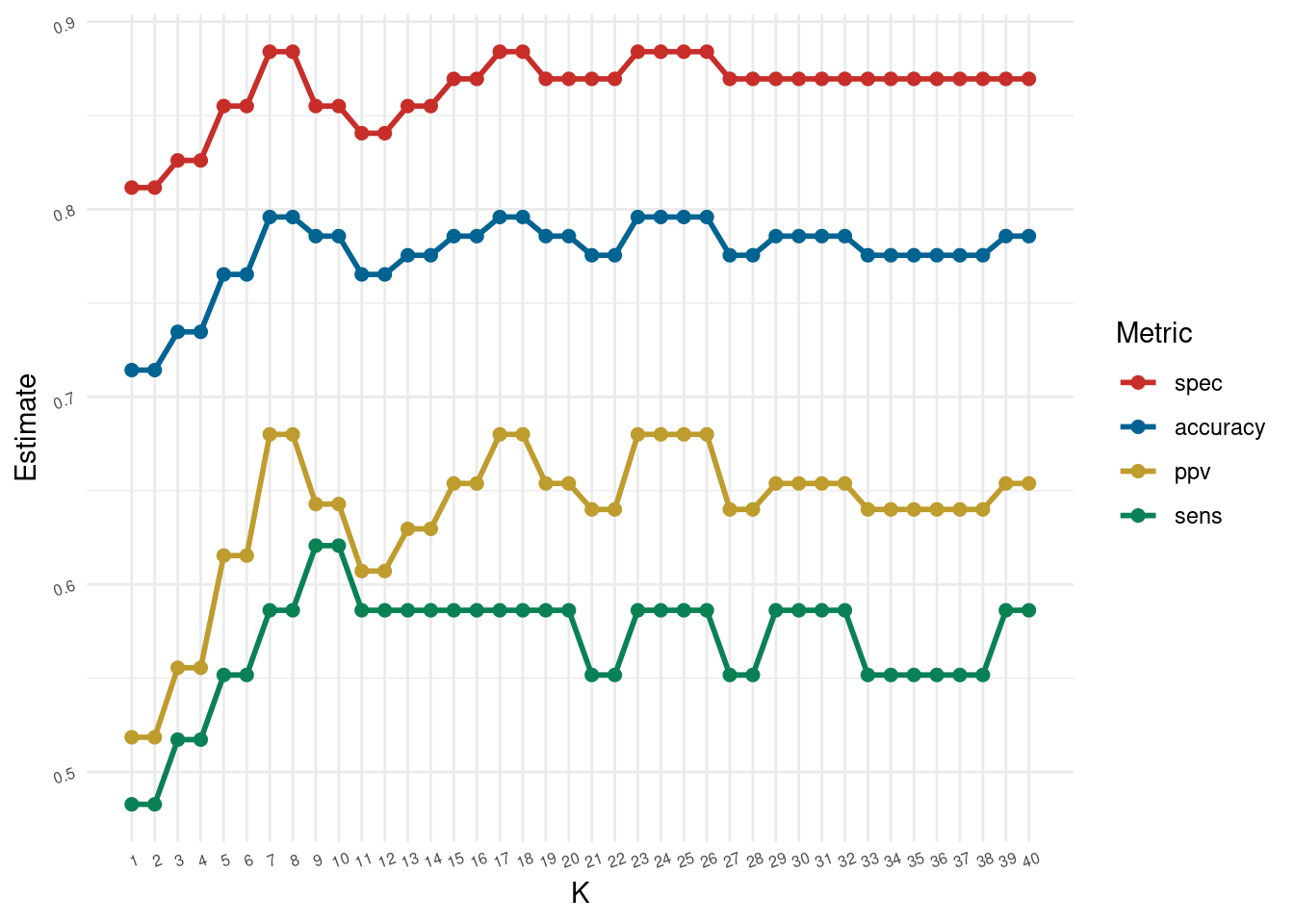
1 ppv binary 0.68Code to recreate the plot in the slides for the diabetes dataset.
Click for answer
Answer:
metrics_for_k <- function(k, db_train, db_test){
db_knn_spec <- nearest_neighbor(mode = "classification",
                             engine = "kknn",
                             weight_func = "rectangular",
                             neighbors = k)

db_knn_wkflow <- workflow() %>%
  add_recipe(db_recipe) %>%
  add_model(db_knn_spec)

db_knn_fit <- fit(db_knn_wkflow, data = db_train)
test_features <- db_test %>% select(glucose, insulin)
nn1_pred <- predict(db_knn_fit, test_features, type = "raw")

db_results <- db_test %>%
  select(diabetes) %>%
  bind_cols(predicted = nn1_pred)
custom_metrics <- metric_set(accuracy, sens, spec, ppv)

metrics <- custom_metrics(db_results,
               truth = diabetes,
               estimate = predicted)
metrics <- metrics %>% select(-.estimator) %>% mutate(k = rep(k,4))

return(list = metrics)
}
k <- seq(1,40, by=1)
optim.results <- purrr::map_dfr(k, ~metrics_for_k(.x, db_train, db_test)) optim.results %>%
ggplot(aes(x = k, y = .estimate, color = forcats::fct_reorder2(.metric, k, .estimate ))) +
geom_line(size = 1) +
geom_point(size = 2) +
theme_minimal() +
ggthemes::scale_color_wsj() +
scale_x_continuous(breaks = k) +
theme(panel.grid.minor.x = element_blank(),
axis.text=element_text(size=6, angle = 20))+
labs(color='Metric', y = "Estimate", x = "K")