# load the necessary libraries
library(tidyverse)
library(tidyr)Class Activity 10
Your Turn 1
students <- tibble(
  id = 1:24,
  grade = sample(c("9th", "10th", "11th"), 24, replace = TRUE),
  region = sample(c("North America", "Europe", "Asia", "South America", "Middle East", "Africa"), 24, replace = TRUE),
  score = round(runif(24,50, 100))
)
a. Create a new column grade_fac by converting the grade column into a factor. Reorder the levels of grade_fac to be “9th”, “10th”, and “11th”. Sort the dataset based on the grade_fac column.
Click for answer
Answer:
students_a <- students %>%
  mutate(grade_fac = factor(grade)) %>%
  mutate(grade_fac = fct_relevel(grade_fac, c("9th", "10th", "11th"))) %>%
  arrange(grade_fac)
print(students_a, n = 24)
# A tibble: 24 × 5
id grade region score grade_fac
<int> <chr> <chr> <dbl> <fct>
1 3 9th Middle East 86 9th
2 4 9th South America 88 9th
3 6 9th South America 82 9th
4 10 9th Europe 69 9th
5 11 9th Asia 77 9th
6 13 9th Europe 87 9th
7 15 9th Europe 97 9th
8 17 9th South America 57 9th
9 2 10th Europe 95 10th
10 7 10th North America 75 10th
11 8 10th Europe 86 10th
12 12 10th Middle East 60 10th
13 14 10th South America 63 10th
14 20 10th Europe 69 10th
15 1 11th Asia 94 11th
16 5 11th North America 59 11th
17 9 11th Africa 63 11th
18 16 11th Middle East 88 11th
19 18 11th Asia 97 11th
20 19 11th Middle East 54 11th
21 21 11th Middle East 75 11th
22 22 11th South America 54 11th
23 23 11th Asia 82 11th
24 24 11th South America 54 11th b. Create a new column region_fac by converting the region column into a factor. Collapse the region_fac levels into three categories: “Americas”, “EMEA” and “Asia”. Count the number of students in each collapsed region category.
c. Create a new column grade_infreq that is a copy of the grade_fac column. Reorder the levels of grade_infreq based on their frequency in the dataset. Print the levels of grade_infreq to check the ordering.
d. Create a new column grade_lumped by lumping the least frequent level of the grade_fac column into an ‘Others’ category. Count the number of students in each of the categories of the grade_lumped column.
Your Turn 2
Lets import the gss_cat dataset from the forcats library. This datast contains a sample of categorical variables from the General Social survey.
# import gss_cat dataset from forcats library
forcats::gss_cat
# A tibble: 21,483 × 9
year marital age race rincome partyid relig denom tvhours
<int> <fct> <int> <fct> <fct> <fct> <fct> <fct> <int>
1 2000 Never married 26 White $8000 to 9999 Ind,near … Prot… Sout… 12
2 2000 Divorced 48 White $8000 to 9999 Not str r… Prot… Bapt… NA
3 2000 Widowed 67 White Not applicable Independe… Prot… No d… 2
4 2000 Never married 39 White Not applicable Ind,near … Orth… Not … 4
5 2000 Divorced 25 White Not applicable Not str d… None Not … 1
6 2000 Married 25 White $20000 - 24999 Strong de… Prot… Sout… NA
7 2000 Never married 36 White $25000 or more Not str r… Chri… Not … 3
8 2000 Divorced 44 White $7000 to 7999 Ind,near … Prot… Luth… NA
9 2000 Married 44 White $25000 or more Not str d… Prot… Other 0
10 2000 Married 47 White $25000 or more Strong re… Prot… Sout… 3
# ℹ 21,473 more rowsUse gss_cat to answer the following questions.
a. Which religions watch the least TV?
Click for answer
Answer:
# your r-code
gss_cat %>%
  drop_na(tvhours) %>%
  group_by(relig) %>%
  summarize(tvhours = mean(tvhours)) %>%
  ggplot(aes(tvhours, fct_reorder(relig, tvhours))) +
    geom_point()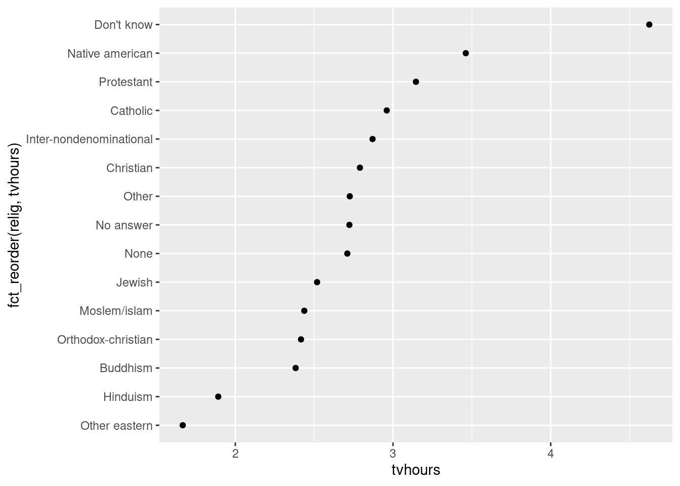
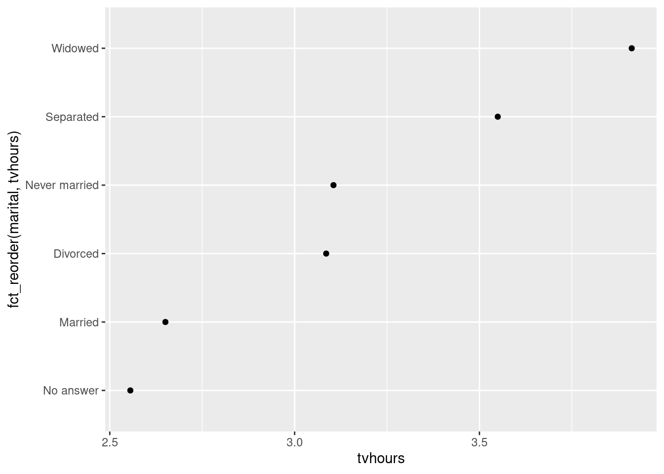
b. Do married people watch more or less TV than single people?
Click for answer
Answer:
# your r-code
gss_cat %>%
  drop_na(tvhours) %>%
  group_by(marital) %>%
  summarize(tvhours = mean(tvhours)) %>%
  ggplot(aes(tvhours, fct_reorder(marital, tvhours))) +
    geom_point()